 Artificial Neural Networks Optimization using Genetic Algorithm with Python
 Artificial Neural Networks Optimization using Genetic Algorithm with Python
This tutorial explains the usage of the genetic algorithm for optimizing the network weights of an Artificial Neural Network for improved performance.

In a previous tutorial titled "Artificial Neural Network Implementation using NumPy and Classification of the Fruits360 Image Dataset" available in my LinkedIn profile at this link https://www.linkedin.com/pulse/artificial-neural-network-implementation-using-numpy-fruits360-gad, an artificial neural network (ANN) is created for classifying 4 classes of the Fruits360 image dataset. The source code used in this tutorial is available in my GitHub page here: https://github.com/ahmedfgad/NumPyANN
A quick summary of this tutorial is extracting the feature vector (360 bins hue channel histogram) and reducing it to just 102 element by using a filter-based technique using the standard deviation. Later, the ANN is built from scratch using NumPy.
The ANN was not completely created as just the forward pass was made ready but there is no backward pass for updating the network weights. This is why the accuracy is very low and not exceeds 45%. The solution to this problem is using an optimization technique for updating the network weights. This tutorial extends the previous one to use the genetic algorithm (GA) for optimizing the network weights.
It is worth-mentioning that both the previous and this tutorial are based on my 2018 book cited as "Ahmed Fawzy Gad 'Practical Computer Vision Applications Using Deep Learning with CNNs'. Dec. 2018, Apress, 978-1-4842-4167-7 ". The book is available at Springer at this link: https://springer.com/us/book/9781484241660. You can find all details within this book.
The source code used in this tutorial is available in my GitHub page here: https://github.com/ahmedfgad/NeuralGenetic
Read More about Genetic Algorithm
Before starting this tutorial, I recommended reading about how the genetic algorithm works and its implementation in Python using NumPy from scratch based on my previous tutorials found at these links:
- Introduction to Optimization with Genetic Algorithm
- https://www.linkedin.com/pulse/introduction-optimization-genetic-algorithm-ahmed-gad/
- https://www.kdnuggets.com/2018/03/introduction-optimization-with-genetic-algorithm.html
- https://towardsdatascience.com/introduction-to-optimization-with-genetic-algorithm-2f5001d9964b
- https://www.springer.com/us/book/9781484241660
- Genetic Algorithm (GA) Optimization - Step-by-Step Example
- Genetic Algorithm Implementation in Python
After understanding how GA works based on numerical examples in addition to implementation using Python, we can start using GA to optimize the ANN by updating its weights (parameters).
Using GA with ANN
GA creates multiple solutions to a given problem and evolves them through a number of generations. Each solution holds all parameters that might help to enhance the results. For ANN, weights in all layers help achieve high accuracy. Thus, a single solution in GA will contain all weights in the ANN. According to the network structure discussed in the previous tutorial and given in the figure below, the ANN has 4 layers (1 input, 2 hidden, and 1 output). Any weight in any layer will be part of the same solution. A single solution to such network will contain a total number of weights equal to 102x150+150x60+60x4=24,540. If the population has 8 solutions with 24,540 parameters per solution, then the total number of parameters in the entire population is 24,540x8=196,320.
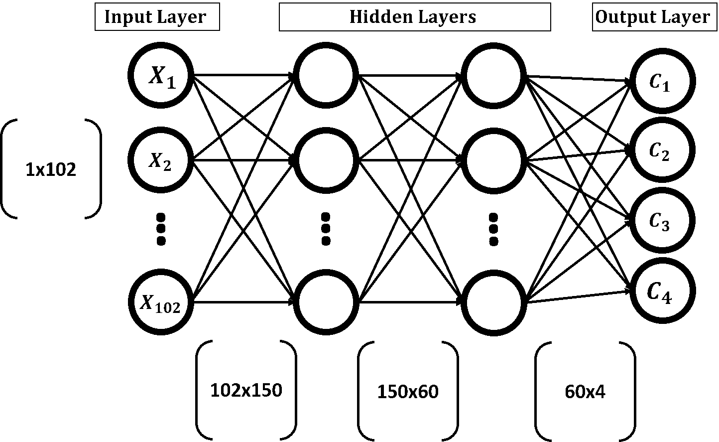
Looking at the above figure, the parameters of the network are in matrix form because this makes calculations of ANN much easier. For each layer, there is an associated weights matrix. Just multiply the inputs matrix by the parameters matrix of a given layer to return the outputs in such layer. Chromosomes in GA are 1D vectors and thus we have to convert the weights matrices into 1D vectors.
Because matrix multiplication is a good option to work with ANN, we will still represent the ANN parameters in the matrix form when using the ANN. Thus, matrix form is used when working with ANN and vector form is used when working with GA. This makes us need to convert the matrix to vector and vice versa. The next figure summarizes the steps of using
GA with ANN. This figure is referred to as the main figure.

Weights Matrices to 1D Vector
Each solution in the population will have two representations. First is a 1D vector for working with GA and second is a matrix to work with ANN. Because there are 3 weights matrices for the 3 layers (2 hidden + 1 output), there will be 3 vectors, one for each matrix. Because a solution in GA is represented as a single 1D vector, such 3 individual 1D vectors will be concatenated into a single 1D vector. Each solution will be represented as a vector of length 24,540. The next Python code creates a function named mat_to_vector() that converts the parameters of all solutions within the population from matrix to vector.
def mat_to_vector(mat_pop_weights):
    pop_weights_vector = []
    for sol_idx in range(mat_pop_weights.shape[0]):
        curr_vector = []
        for layer_idx in range(mat_pop_weights.shape[1]):
            vector_weights = numpy.reshape(mat_pop_weights[sol_idx, layer_idx], newshape=(mat_pop_weights[sol_idx, layer_idx].size))
            curr_vector.extend(vector_weights)
        pop_weights_vector.append(curr_vector)
    return numpy.array(pop_weights_vector)
The function accepts an argument representing the population of all solutions in order to loop through them and return their vector representation. At the beginning of the function, an empty list variable named pop_weights_vector is created to hold the result (vectors of all solutions). For each solution in matrix form, there is an inner loop that loops through its three matrices. For each matrix, it is converted into a vector using the numpy.reshape() function which accepts the input matrix and the output size to which the matrix will be reshaped. The variable curr_vector accepts all vectors for a single solution. After all vectors are generated, they get appended into the pop_weights_vector variable.
Note that we used the numpy.extend() function for vectors belonging to the same solution and numpy.append() for vectors belonging to different solutions. The reason is that numpy.extend() takes the numbers within the 3 vectors belonging to the same solution and concatenate them together. In other words, calling this function for two lists returns a new single list with numbers from both lists. This is suitable in order to create just a 1D chromosome for each solution. But numpy.append() will return three lists for each solution. Calling it for two lists, it returns a new list which is split into two sub-lists. This is not our objective. Finally, the function mat_to_vector() returns the population solutions as a NumPy array for easy manipulation later.
Implementing GA Steps
After converting all solutions from matrices to vectors and concatenated together, we are ready to go through the GA steps discussed in the tutorial titled "Introduction to Optimization with Genetic Algorithm". The steps are presented in the main figure and also summarized in the next figure.
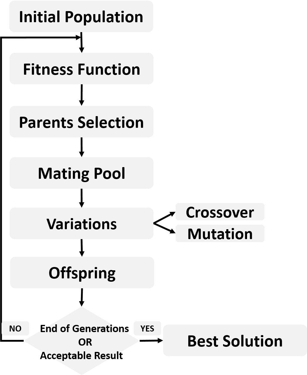
Remember that GA uses a fitness function to returns a fitness value for each solution. The higher the fitness value the better the solution. The best solutions are returned as parents in the parents selection step.
One of the common fitness functions for a classifier such as ANN is the accuracy. It is the ratio between the correctly classified samples and the total number of samples. It is calculated according to the next equation. The classification accuracy of each solution is calculated according to steps in the main figure.

The single 1D vector of each solution is converted back into 3 matrices, one matrix for each layer (2 hidden and 1 output). Conversion takes place using a function called vector_to_mat(). It is defined in the next code.
def vector_to_mat(vector_pop_weights, mat_pop_weights):

    mat_weights = []

    for sol_idx in range(mat_pop_weights.shape[0]):

        start = 0

        end = 0

        for layer_idx in range(mat_pop_weights.shape[1]):

            end = end + mat_pop_weights[sol_idx, layer_idx].size

            curr_vector = vector_pop_weights[sol_idx, start:end]

            mat_layer_weights = numpy.reshape(curr_vector, newshape=(mat_pop_weights[sol_idx, layer_idx].shape))

            mat_weights.append(mat_layer_weights)

            start = end

    return numpy.reshape(mat_weights, newshape=mat_pop_weights.shape)
It reverses the work done previously. But there is an important question. If the vector of a given solution is just one piece, how we can split into three different parts, each part represents a matrix? The size of the first parameters matrix between the input layer and the hidden layer is 102x150. When being converted into a vector, its length will be 15,300. Because it is the first vector to be inserted in the curr_vector variable according to the mat_to_vector() function, then its indices start from index 0 and end at index 15,299. The mat_pop_weights is used as an argument for the vector_to_mat() function in order to know the size of each matrix. We are not interested in using the weights from the mat_pop_weights variable but just the matrices sizes are used from it.
For the second vector in the same solution, it will be the result of converting a matrix of size 150x60. Thus the vector length is 9,000. Such a vector is inserted into the curr_vector variable just before the previous vector of length 15,300. As a result, it will start from index 15,300 and ends at index 15,300+9,000-1=24,299. The -1 is used because Python starts indexing at 0. For the last vector created from the parameters matrix of size 60x4, its length is 240. Because it is added into the curr_vector variable exactly after the previous vector of length 9,000, then its index will start after it. That is its start index is 24,300 and its end index is 24,300+240-1=24,539. So, we can successfully restore the vector into the original 3 matrices.
The matrices returned for each solution are used to predict the class label for each of the 1,962 samples in the used dataset to calculate the accuracy. This is done using 2 functions which are predict_outputs() and fitness() according to the next code.
def predict_outputs(weights_mat, data_inputs, data_outputs, activation="relu"):

    predictions = numpy.zeros(shape=(data_inputs.shape[0]))

    for sample_idx in range(data_inputs.shape[0]):

        r1 = data_inputs[sample_idx, :]

        for curr_weights in weights_mat:

            r1 = numpy.matmul(a=r1, b=curr_weights)

            if activation == "relu":

                r1 = relu(r1)

            elif activation == "sigmoid":

                r1 = sigmoid(r1)

        predicted_label = numpy.where(r1 == numpy.max(r1))[0][0]

        predictions[sample_idx] = predicted_label

    correct_predictions = numpy.where(predictions == data_outputs)[0].size

    accuracy = (correct_predictions/data_outputs.size)*100

    return accuracy, predictions


def fitness(weights_mat, data_inputs, data_outputs, activation="relu"):

    accuracy = numpy.empty(shape=(weights_mat.shape[0]))

    for sol_idx in range(weights_mat.shape[0]):

        curr_sol_mat = weights_mat[sol_idx, :]

        accuracy[sol_idx], _ = predict_outputs(curr_sol_mat, data_inputs, data_outputs, activation=activation)

    return accuracy
The predict_outputs() function accepts the weights of a single solution, inputs, and outputs of the training data, and an optional parameter that specifies which activation function to use. It returns the accuracy of just one solution not all solutions within the population. It order to return the fitness value (i.e. accuracy) of all solutions within the population, the fitness() function loops through each solution, pass it to the predict_outputs() function, store the accuracy of all solutions into the accuracy array, and finally return such an array.
After calculating the fitness value (i.e. accuracy) for all solutions, the remaining steps of GA in the main figure are applied the same way done previously. The best parents are selected, based on their accuracy, into the mating pool. Then mutation and crossover variants are applied in order to produce the offspring. The population of the new generation is created using both offspring and parents. These steps are repeated for a number of generations.