Naive Bayes: A Baseline Model for Machine Learning Classification Performance
We can use Pandas to conduct Bayes Theorem and Scikitlearn to implement the Naive Bayes Algorithm. We take a step by step approach to understand Bayes and implementing the different options in Scikitlearn.
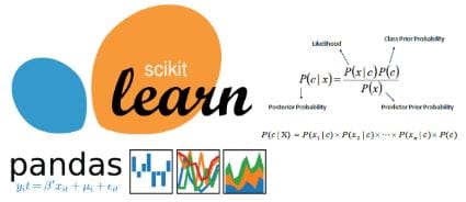
Bayes Theorem

The above equation represents Bayes Theorem in which it describes the probability of an event occurring P(A) based on our prior knowledge of events that may be related to that event P(B).
Lets explore the parts of Bayes Theorem:
- P(A|B) - Posterior Probability
- The conditional probability that event A occurs given that event B has occurred.
- P(A) - Prior Probability
- The probability of event A.
- P(B) - Evidence
- The probability of event B.
- P(B|A) - Likelihood
- The conditional probability of B occurring given event A has occurred.
Now, lets explore the parts of Bayes Theorem through the eyes of someone conducting machine learning:
- P(A|B) - Posterior Probability
- The conditional probability of the response variable (target variable) given the training data inputs.
- P(A) - Prior Probability
- The probability of the response variable (target variable).
- P(B) - Evidence
- The probability of the training data.
- P(B|A) - Likelihood
- The conditional probability of the training data given the response variable.
- P(c|x) - Posterior probability of the target/class (c) given predictors (x).
- P(c) - Prior probability of the class (target).
- P(x|c) - Probability of the predictor (x) given the class/target (c).
- P(x) - Prior probability of the predictor (x).
Example of using Bayes theorem:
I'll be using the tennis weather dataset.
import numpy as np
import pandas as pd
import matplotlib.pyplot as plt
%matplotlib inline
tennis = pd.read_csv('tennis.csv')
tennis
| outlook | temp | humidity | windy | play | |
|---|---|---|---|---|---|
| 0 | sunny | hot | high | False | no |
| 1 | sunny | hot | high | True | no |
| 2 | overcast | hot | high | False | yes |
| 3 | rainy | mild | high | False | yes |
| 4 | rainy | cool | normal | False | yes |
| 5 | rainy | cool | normal | True | no |
| 6 | overcast | cool | normal | True | yes |
| 7 | sunny | mild | high | False | no |
| 8 | sunny | cool | normal | False | yes |
| 9 | rainy | mild | normal | False | yes |
| 10 | sunny | mild | normal | True | yes |
| 11 | overcast | mild | high | True | yes |
| 12 | overcast | hot | normal | False | yes |
| 13 | rainy | mild | high | True | no |
Lets take a look at how each category looks when inside a frequency table:
outlook = tennis.groupby(['outlook', 'play']).size()
temp = tennis.groupby(['temp', 'play']).size()
humidity = tennis.groupby(['humidity', 'play']).size()
windy = tennis.groupby(['windy', 'play']).size()
play = tennis.play.value_counts()
print(temp)
print('------------------')
print(humidity)
print('------------------')
print(windy)
print('------------------')
print(outlook)
print('------------------')
print('play')
print(play)
temp  play
cool  no      1
      yes     3
hot   no      2
      yes     2
mild  no      2
      yes     4
dtype: int64
------------------
humidity  play
high      no      4
          yes     3
normal    no      1
          yes     6
dtype: int64
------------------
windy  play
False  no      2
       yes     6
True   no      3
       yes     3
dtype: int64
------------------
outlook   play
overcast  yes     4
rainy     no      2
          yes     3
sunny     no      3
          yes     2
dtype: int64
------------------
play
yes    9
no     5
Name: play, dtype: int64
What is the probability of playing tennis given it is rainy?
- P(rain|play=yes)
- frequency of (outlook=rainy) when (play=yes) / frequency of (play=yes) = 3/9
- P(play=yes)
- frequency of (play=yes) / total(play) = 9/14
- P(outlook=rainy)
- frequency of (outlook=rainy) / total(outlook) = 5/14

(3/9)*(9/14)/(5/14)
0.6
The probability of playing tennis when it is rainy is 60%. The process is very simple once you obtain the frequencies for each category.
Here is a simple function to help any newbies remember the parts of Bayes equation:
  def bayestheorem():
    print('Posterior [P(c|x)] - Posterior probability of the target/class (c) given predictors (x)'),
    print('Prior [P(c)] - Prior probability of the class (target)'),
    print('Likelihood [P(x|c)] - Probability of the predictor (x) given the class/target (c)'),
    print('Evidence [P(x)] - Prior probability of the predictor (x))')
Here is a simple function to calculate the posterior probability for you, but you must be able to find each part of bayes equation yourself.
  def bayesposterior(prior, likelihood, evidence, string):
      print('Prior=', prior),
      print('Likelihood=', likelihood),
      print('Evidence=', evidence),
      print('Equation =','(Prior*Likelihood)/Evidence')
      print(string, (prior*likelihood)/evidence)
Lets see another way to find the posterior probability this time using contingency tables in Python:
ct = pd.crosstab(tennis['outlook'], tennis['play'], margins = True)
print(ct)
          no  yes  rowtotal
overcast   0    4         4
rainy      2    3         5
sunny      3    2         5
coltotal   5    9        14
ct.columns = ["no","yes","rowtotal"]
ct.index= ["overcast","rainy","sunny","coltotal"]
ct / ct.loc["coltotal","rowtotal"]
| no | yes | rowtotal | |
|---|---|---|---|
| overcast | 0.000000 | 0.285714 | 0.285714 |
| rainy | 0.142857 | 0.214286 | 0.357143 |
| sunny | 0.214286 | 0.142857 | 0.357143 |
| coltotal | 0.357143 | 0.642857 | 1.000000 |
To only get the column total
ct / ct.loc["coltotal"]
| no | yes | rowtotal | |
|---|---|---|---|
| overcast | 0.0 | 0.444444 | 0.285714 |
| rainy | 0.4 | 0.333333 | 0.357143 |
| sunny | 0.6 | 0.222222 | 0.357143 |
| coltotal | 1.0 | 1.000000 | 1.000000 |
To only get the row total
ct.div(ct["rowtotal"], axis=0)
| no | yes | rowtotal | |
|---|---|---|---|
| overcast | 0.000000 | 1.000000 | 1.0 |
| rainy | 0.400000 | 0.600000 | 1.0 |
| sunny | 0.600000 | 0.400000 | 1.0 |
| coltotal | 0.357143 | 0.642857 | 1.0 |
These tables are all pandas dataframe objects. Therefore using pandas subsetting and the bayesposterior function I made, we can arrive at the same conclusion:
bayesposterior(prior = ct.iloc[1,1]/ct.iloc[3,1],
               likelihood = ct.iloc[3,1]/ct.iloc[3,2],
               evidence = ct.iloc[1,2]/ct.iloc[3,2],
               string = 'Probability of Tennis given Rain =')
Prior= 0.3333333333333333
Likelihood= 0.6428571428571429
Evidence= 0.35714285714285715
Equation = (Prior*Likelihood)/Evidence
Probability of Tennis given Rain = 0.6
Naive Bayes Algorithm
Naive Bayes is a supervised Machine Learning algorithm inspired by the Bayes theorem. It works on the principles of conditional probability. Naive Bayes is a classification algorithm for binary and multi-class classification. The Naive Bayes algorithm uses the probabilities of each attribute belonging to each class to make a prediction.
Example
What is the probability of playing tennis when it is sunny, hot, highly humid and windy? So using the tennis dataset, we need to use the Naive Bayes method to predict the probability of someone playing tennis given the mentioned weather conditions.
pd.crosstab(tennis['outlook'], tennis['play'], margins = True)
| play | no | yes | All |
|---|---|---|---|
| outlook | |||
| overcast | 0 | 4 | 4 |
| rainy | 2 | 3 | 5 |
| sunny | 3 | 2 | 5 |
| All | 5 | 9 | 14 |
pd.crosstab(tennis['temp'], tennis['play'], margins = True)
| play | no | yes | All |
|---|---|---|---|
| temp | |||
| cool | 1 | 3 | 4 |
| hot | 2 | 2 | 4 |
| mild | 2 | 4 | 6 |
| All | 5 | 9 | 14 |
pd.crosstab(tennis['humidity'], tennis['play'], margins = True)
| play | no | yes | All |
|---|---|---|---|
| humidity | |||
| high | 4 | 3 | 7 |
| normal | 1 | 6 | 7 |
| All | 5 | 9 | 14 |
pd.crosstab(tennis['windy'], tennis['play'], margins = True)
| play | no | yes | All |
|---|---|---|---|
| windy | |||
| False | 2 | 6 | 8 |
| True | 3 | 3 | 6 |
| All | 5 | 9 | 14 |
pd.crosstab(index=tennis['play'],columns="count", margins=True)
| col_0 | count | All |
|---|---|---|
| play | ||
| no | 5 | 5 |
| yes | 9 | 9 |
| All | 14 | 14 |
Now by using the above contingency tables, we will go through how the Naive Bayes algorithm calculates the posterior probability.
-
- Calculate P(x|play=yes). In this case x refers to all the predictors 'outlook', 'temp', 'humidity' and 'windy'.
- P(sunny|play=yes)→2/9
- P(hot|play=yes)→2/9
- P(high|play=yes)→3/9
- P(True|play=yes)→3/9
- Calculate P(x|play=yes). In this case x refers to all the predictors 'outlook', 'temp', 'humidity' and 'windy'.

p_x_yes = ((2/9)*(2/9)*(3/9)*(3/9))
print('The probability of the predictors given playing tennis is', '%.3f'%p_x_yes)
The probability of the predictors given playing tennis is 0.005
-
- Calculate P(x|play=no) using the same method as above.
- P(sunny|play=no)→3/5
- P(hot|play=no)→2/5
- P(high|play=no)→4/5
- P(True|play=no)→3/5
- Calculate P(x|play=no) using the same method as above.
p_x_no = ((3/5)*(2/5)*(4/5)*(3/5))
print('The probability of the predictors given not playing tennis is ', '%.3f'%p_x_no)
The probability of the predictors given not playing tennis is 0.115
-
- Calculate P(play=yes) and P(play=no)
- P(play=yes)→9/14
- P(play=yes)→5/14
- Calculate P(play=yes) and P(play=no)
yes = (9/14)
no = (5/14)
print('The probability of playing tennis is', '%.3f'% yes)
print('The probability of not playing tennis is', '%.3f'% no)
The probability of playing tennis is 0.643
The probability of not playing tennis is 0.357
-
- Calculate the probability of playing and not playing tennis given the predictors

yes_x = p_x_yes*yes
print('The probability of playing tennis given the predictors is', '%.3f'%yes_x)

no_x = p_x_no*no
print('The probability of not playing tennis given the predictors is', '%.3f'%no_x)
  The probability of playing tennis given the predictors is 0.004
  The probability of not playing tennis given the predictors is 0.041
-
- The prediction will be whichever probability is higher
if yes_x > no_x:
  print('The probability of playing tennis when the outlook is sunny, the temperature is hot, there is high humidity and windy is higher')
else:
  print('The probability of not playing tennis when the outlook is sunny, the temperature is hot, there is high humidity and windy is higher')
The probability of not playing tennis is higher when the outlook is sunny, the temperature is hot, there is high humidity and it is windy.
Type of Naive Bayes Algorithm
Python's Scikitlearn gives the user access to the following 3 Naive Bayes models.
- Gaussian
- The gaussian NB Alogorithm assumes all contnuous features (predictors) and all follow a Gaussian (Normal Distribution).
- Multinomial
- Multinomial NB is suited for discrete data that have frequencies and counts. Spam Filtering and Text/Document Classification are two very well-known use cases.
- Bernoulli
- Bernoulli is similar to Multinomial except it is for boolean/binary features. Like the multinomial method it can be used for spam filtering and document classification in which binary terms (i.e. word occurrence in a document represented with True or False).
Lets implement a Multinomial and Gaussian Model with Scikitlearn
from sklearn.naive_bayes import GaussianNB, BernoulliNB, MultinomialNB
from sklearn.model_selection import train_test_split
from sklearn.metrics import *