Who is your Golden Goose?: Cohort Analysis

comments

By Jiwon Jeong, a Graduate Research Assistant at Yonsei University

Customer segmentation is the technique of dividing customers into groups based on their purchase patterns to identify who are the most profitable groups. In segmenting customers, various criteria can also be used depending on the market such as geographic, demographic characteristics or behavior bases. This technique assumes that groups with different features require different approaches to marketing and wants to figure out the groups who can boost their profitability the most.

Today, we are going to discuss how to do customer segmentation analysis with the online retail dataset from UCI ML repo. This analysis will be focused on two steps getting the RFM values and making clusters with K-means algorithms. The dataset and the full code is also available on my Github. The original resource of this note is from the course “Customer Segmentation Analysis in Python.”

What is RFM?

RFM is an acronym of recency, frequency and monetary. Recency is about when was the last order of a customer. It means the number of days since a customer made the last purchase. If it’s a case for a website or an app, this could be interpreted as the last visit day or the last login time.

Frequency is about the number of purchase in a given period. It could be 3 months, 6 months or 1 year. So we can understand this value as for how often or how many a customer used the product of a company. The bigger the value is, the more engaged the customers are. Could we say them as our VIP? Not necessary. Cause we also have to think about how much they actually paid for each purchase, which means monetary value.

Monetary is the total amount of money a customer spent in that given period. Therefore big spenders will be differentiated with other customers such as MVP or VIP.

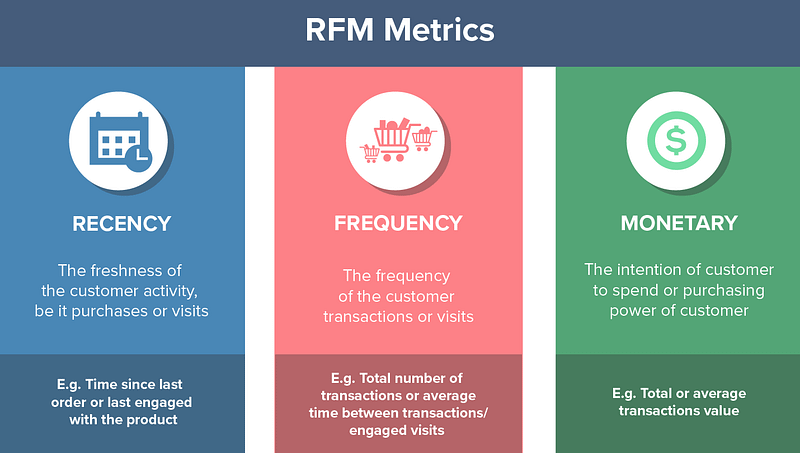
Photo from CleverTap

These three values are commonly used quantifiable factors in cohort analysis. Because of their simple and intuitive concept, they are popular among other customer segmentation methods.

Import the data

So we are going to apply RFM to our cohort analysis today. The dataset we are going to use is the transaction history data occurring from Jan 2010 to Sep 2011. As this is a tutorial guideline for cohort analysis, I’m going to use only the randomly selected fraction of the original dataset.

# Import data
online = pd.read_excel('Online Retail.xlsx')
# drop the row missing customer ID 
online = online[online.CustomerID.notnull()]
online = online.sample(frac = .3).reset_index(drop = True)
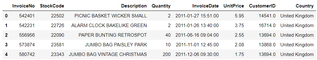
online.head()

Calculating RFM values

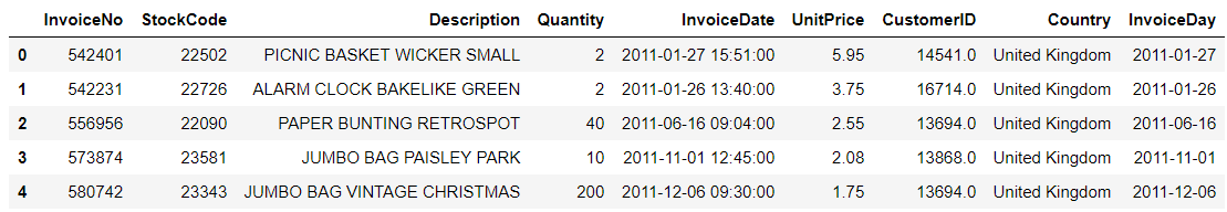
The first thing we’re going to count is the recency value, the number of days since the last order of a customer. From which column could we get that value? InvoiceData. With this column, we can get when was the first purchase and when was the last purchase of a customer. Let’s call the first one as CohortDay. As InvoiceDate also contains additional time data, we need to extract the year, month and day part. After that, we’ll get CohortDay which is the minimum of InvoiceDay.

# extract year, month and day
online['InvoiceDay'] = online.InvoiceDate.apply(lambda x: dt.datetime(x.year, x.month, x.day))
online.head()

As we randomly chose the subset of the data, we also need to know the time period of our data. Like what you can see below, the final day of our dataset is December 9th, 2011. Therefore set December 10th as our pining date and count backward the number of days from the latest purchase for each customer. That will be the recency value.

 # print the time period
print('Min : {}, Max : {}'.format(min(online.InvoiceDay), max(online.InvoiceDay)))

# pin the last date
pin_date = max(online.InvoiceDay) + dt.timedelta(1)

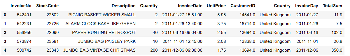
Before getting the recency, let’s count one more value in advance, the total amount of money each customer spent. This is for counting the monetary value. How can we get that? Easy! Multiplying the product price and the quantity of the order in each row.

# Create total spend dataframe
online['TotalSum'] = online.Quantity * online.UnitPrice
online.head()

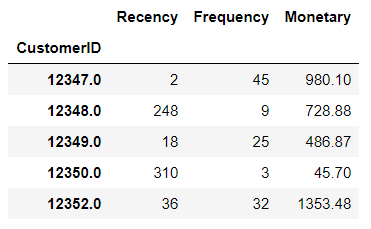
Now we are ready to get the three RFM values at once. I’ll group the data for each customer and aggregate it for each recency, frequency, and monetary value.

# calculate RFM values
rfm = online.groupby('CustomerID').agg({
    'InvoiceDate' : lambda x: (pin_date - x.max()).days,
    'InvoiceNo' : 'count', 
    'TotalSum' : 'sum'})
# rename the columns
rfm.rename(columns = {'InvoiceDate' : 'Recency', 
                      'InvoiceNo' : 'Frequency', 
                      'TotalSum' : 'Monetary'}, inplace = True)
rfm.head()

RFM quartiles

Now we’ll group the customers based on RFM values. Cause these are continuous values, we can also use the quantile values and divide them into 4 groups.

# create labels and assign them to tree percentile groups 
r_labels = range(4, 0, -1)
r_groups = pd.qcut(rfm.Recency, q = 4, labels = r_labels)
f_labels = range(1, 5)
f_groups = pd.qcut(rfm.Frequency, q = 4, labels = f_labels)
m_labels = range(1, 5)
m_groups = pd.qcut(rfm.Monetary, q = 4, labels = m_labels)

Please pay extra care for the r_labels. I gave the labels in descending order. Why is that? Because recency means how much time has elapsed since a customer’s last order. Therefore the smaller the value is, the more engaged a customer to that brand. Now let’s make a new column for indicating group labels.

# make a new column for group labels
rfm['R'] = r_groups.values
rfm['F'] = f_groups.values
rfm['M'] = m_groups.values
# sum up the three columns
rfm['RFM_Segment'] = rfm.apply(lambda x: str(x['R']) + str(x['F']) + str(x['M']), axis = 1)
rfm['RFM_Score'] = rfm[['R', 'F', 'M']].sum(axis = 1)
rfm.head()

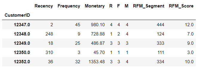
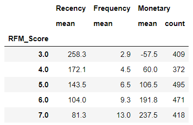
I attached all three labels in one cell as RFM_Segment. In this way, we can easily check what level or segment a customer belongs to. RFM_Score is the total sum of the three values. It doesn’t necessarily have to be the sum so the mean value is also possible. Moreover, we can catch further patterns with the mean or count values of recency, frequency and monetary grouped by this score like below.

# calculate average values for each RFM
rfm_agg = rfm.groupby('RFM_Score').agg({
    'Recency' : 'mean',
    'Frequency' : 'mean',
    'Monetary' : ['mean', 'count']
})
rfm_agg.round(1).head()

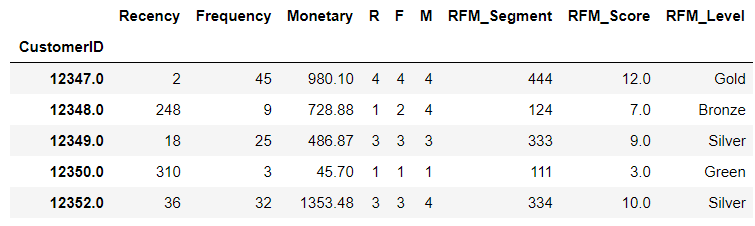
RFM_Score will be the total score of a customer’s engagement or loyalty. Summing up the three values altogether, we can finally categorize customers into ‘Gold,’ ‘Silver,’ ‘Bronze,’ and ‘Green’.

# assign labels from total score
score_labels = ['Green', 'Bronze', 'Silver', 'Gold']
score_groups = pd.qcut(rfm.RFM_Score, q = 4, labels = score_labels)
rfm['RFM_Level'] = score_groups.values
rfm.head()

Great! We’re done with one cohort analysis with RFM values. We identified who is our golden goose and where we should take extra care. Now why don’t we try a different method for customer segmentation and compare the two results?