Modeling Price with Regularized Linear Model & XGBoost
We are going to implement regularization techniques for linear regression of house pricing data. Our goal in price modeling is to model the pattern and ignore the noise.
By Susan Li, Sr. Data Scientist
We would like to model the price of a house, we know that the price depends on the location of the house, square footage of a house, year built, year renovated, number of bedrooms, number of garages, etc. So those factors contribute to the pattern — premium location would typically lead to a higher price. However, all houses within the same area and have same square footage do not have the exact same price. The variation in price is the noise. Our goal in price modeling is to model the pattern and ignore the noise. The same concepts apply to modeling hotel room prices too.
Therefore, to start, we are going to implement regularization techniques for linear regression of house pricing data.
The Data
There is an excellent house prices data set can be found here.
import warnings
def ignore_warn(*args, **kwargs):
pass
warnings.warn = ignore_warn
import numpy as np
import pandas as pd
%matplotlib inline
import matplotlib.pyplot as plt
import seaborn as sns
from scipy import stats
from scipy.stats import norm, skew
from sklearn import preprocessing
from sklearn.metrics import r2_score
from sklearn.metrics import mean_squared_error
from sklearn.model_selection import train_test_split
from sklearn.linear_model import ElasticNetCV, ElasticNet
from xgboost import XGBRegressor, plot_importance
from sklearn.model_selection import RandomizedSearchCV
from sklearn.model_selection import StratifiedKFold
pd.set_option('display.float_format', lambda x: '{:.3f}'.format(x))
df = pd.read_csv('house_train.csv')
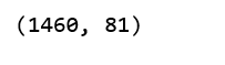
df.shape
(df.isnull().sum() / len(df)).sort_values(ascending=False)[:20]
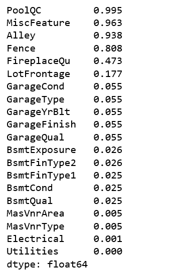
The good news is that we have many features to play with (81), the bad news is that 19 features have missing values, and 4 of them have over 80% missing values. For any feature, if it is missing 80% of values, it can’t be that important, therefore, I decided to remove these 4 features.
df.drop(['PoolQC', 'MiscFeature', 'Alley', 'Fence', 'Id'], axis=1, inplace=True)
Explore Features
Target feature distribution
sns.distplot(df['SalePrice'] , fit=norm);

# Get the fitted parameters used by the function
(mu, sigma) = norm.fit(df['SalePrice'])
print( '\n mu = {:.2f} and sigma = {:.2f}\n'.format(mu, sigma))

# Now plot the distribution
plt.legend(['Normal dist. ($\mu=$ {:.2f} and $\sigma=$ {:.2f} )'.format(mu, sigma)],
            loc='best')
plt.ylabel('Frequency')
plt.title('Sale Price distribution')

# Get also the QQ-plot
fig = plt.figure()
res = stats.probplot(df['SalePrice'], plot=plt)
plt.show();
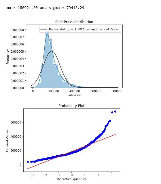
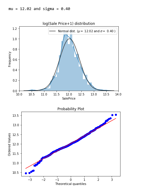
The target feature - SalePrice is right skewed. As linear models like normally distributed data , we will transform SalePrice and make it more normally distributed.
sns.distplot(np.log1p(df['SalePrice']) , fit=norm);

# Get the fitted parameters used by the function
(mu, sigma) = norm.fit(np.log1p(df['SalePrice']))
print( '\n mu = {:.2f} and sigma = {:.2f}\n'.format(mu, sigma))

# Now plot the distribution
plt.legend(['Normal dist. ($\mu=$ {:.2f} and $\sigma=$ {:.2f} )'.format(mu, sigma)],
            loc='best')
plt.ylabel('Frequency')
plt.title('log(Sale Price+1) distribution')

# Get also the QQ-plot
fig = plt.figure()
res = stats.probplot(np.log1p(df['SalePrice']), plot=plt)
plt.show();
Correlation between numeric features
pd.set_option('precision',2)
plt.figure(figsize=(10, 8))
sns.heatmap(df.drop(['SalePrice'],axis=1).corr(), square=True)
plt.suptitle("Pearson Correlation Heatmap")
plt.show();
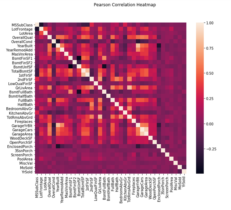
There exists strong correlations between some of the features. For example, GarageYrBlt and YearBuilt, TotRmsAbvGrd and GrLivArea, GarageArea and GarageCars are strongly correlated. They actually express more or less the same thing. I will let ElasticNetCV to help reduce redundancy later.
Correlation between SalePrice and the other numeric features
corr_with_sale_price = df.corr()["SalePrice"].sort_values(ascending=False)
plt.figure(figsize=(14,6))
corr_with_sale_price.drop("SalePrice").plot.bar()
plt.show();
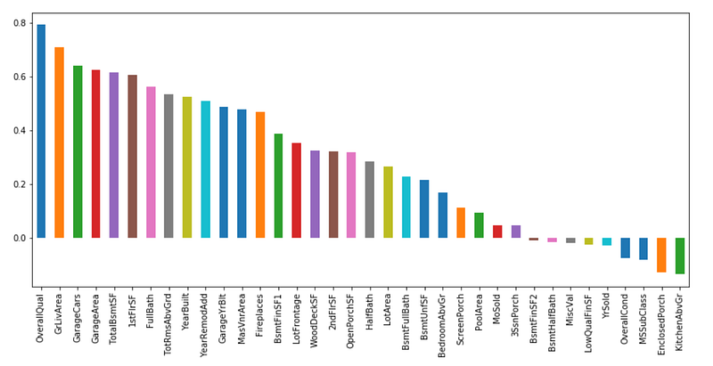
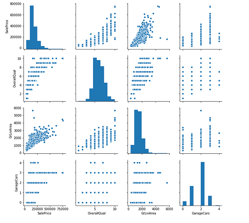
The correlation of SalePrice with OverallQual is the greatest (around 0.8). Also GrLivArea presents a correlation of over 0.7, and GarageCars presents a correlation of over 0.6. Let’s look at these 4 features in more detail.
sns.pairplot(df[['SalePrice', 'OverallQual', 'GrLivArea', 'GarageCars']])
plt.show();
Feature Engineering
- Log transform features that have a highly skewed distribution (skew > 0.75)
- Dummy coding categorical features
- Fill NaN with the mean of the column.
- Train and test sets split.
feature_engineering_price.py
ElasticNet
- Ridge and Lasso regression are regularized linear regression models.
- ElasticNet is essentially a Lasso/Ridge hybrid, that entails the minimization of an objective function that includes both L1 (Lasso) and L2(Ridge) norms.
- ElasticNet is useful when there are multiple features which are correlated with one another.
- The class ElasticNetCV can be used to set the parameters
alpha(α) andl1_ratio(ρ) by cross-validation. - ElasticNetCV: ElasticNet model with best model selection by cross-validation.
Let’s see what ElasticNetCV is going to select for us.
ElasticNetCV.py
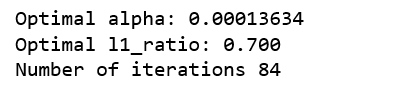
Figure 8
0< The optimal l1_ratio <1 , indicating the penalty is a combination of L1 and L2, that is, the combination of Lasso and Ridge.
Model Evaluation
ElasticNetCV_evaluation.py
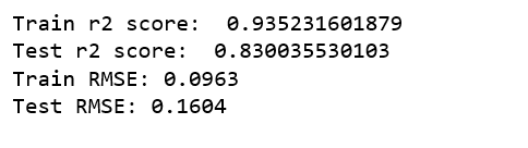
The RMSE here is actually RMSLE ( Root Mean Squared Logarithmic Error). Because we have taken the log of the actual values. Here is a nice write up explaining the differences between RMSE and RMSLE.
Feature Importance
feature_importance = pd.Series(index = X_train.columns, data = np.abs(cv_model.coef_))

n_selected_features = (feature_importance>0).sum()
print('{0:d} features, reduction of {1:2.2f}%'.format(
    n_selected_features,(1-n_selected_features/len(feature_importance))*100))

feature_importance.sort_values().tail(30).plot(kind = 'bar', figsize = (12,5));
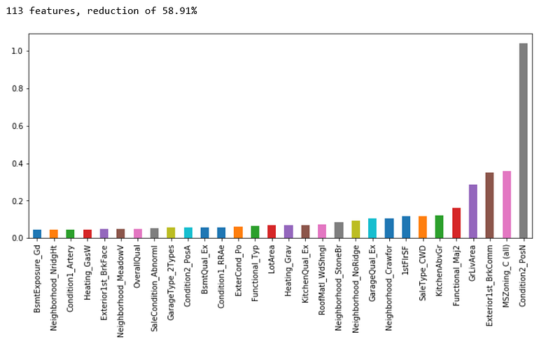
A reduction of 58.91% features looks productive. The top 4 most important features selected by ElasticNetCV are Condition2_PosN, MSZoning_C(all), Exterior1st_BrkComm & GrLivArea. We are going to see how these features compare with those selected by Xgboost.
Xgboost
The first Xgboost model, we start from default parameters.
xgb_model1.py
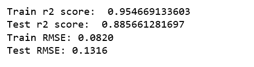
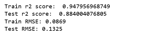
It is already way better an the model selected by ElasticNetCV!
The second Xgboost model, we gradually add a few parameters that suppose to add model’s accuracy.
xgb_model2.py
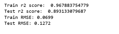
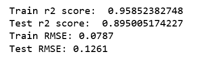
There was again an improvement!
The third Xgboost model, we add a learning rate, hopefully it will yield a more accurate model.
xgb_model3.py
Unfortunately, there was no improvement. I concluded that xgb_model2 is the best model.
Feature Importance
from collections import OrderedDict
OrderedDict(sorted(xgb_model2.get_booster().get_fscore().items(), key=lambda t: t[1], reverse=True))
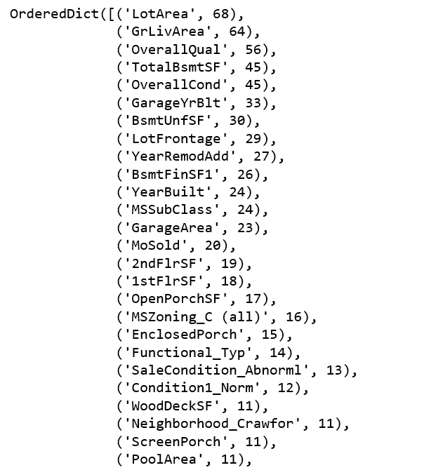
The top 4 most important features selected by Xgboost are LotArea, GrLivArea, OverallQual & TotalBsmtSF.
There is only one feature GrLivArea was selected by both ElasticNetCV and Xgboost.
So now we are going to select some relevant features and fit the Xgboost again.
xgb_model5.py
Another small improvement!
Jupyter notebook can be found on Github. Enjoy the rest of the week!
Bio: Susan Li is changing the world, one article at a time. She is a Sr. Data Scientist, located in Toronto, Canada.
Original. Reposted with permission.
Related:
- Unveiling Mathematics Behind XGBoost
- Multi-Class Text Classification with Scikit-Learn
- An Introduction on Time Series Forecasting with Simple Neural Networks & LSTM