 Unveiling Mathematics Behind XGBoost
 Unveiling Mathematics Behind XGBoost
Follow me till the end, and I assure you will atleast get a sense of what is happening underneath the revolutionary machine learning model.
By Ajit Samudrala, Aspiring Data Scientist
This article is targeted at people who found it difficult to grasp the original paper. Follow me till the end, and I assure you will at least get a sense of what is happening underneath the revolutionary machine learning model. Lets get started.
Curious case of John and Emily

John and Emily embarked on an adventure to pluck apples from the tree located at the lowest point of the mountain. While Emily is a smart and adventurous girl, John is a bit cautious and sluggish. However, only John can climb tree and pluck apples. We will see how they achieve their goal.
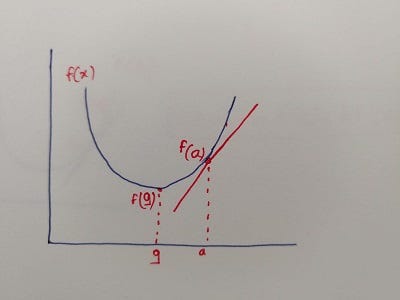
John and Emily start at point ‘a’ on the mountain and tree is located at point ‘g’. There are two ways they can reach point ‘g’:
1. Emily calculates the slope of the curve at point ‘a’; if the slope is positive, they move in the opposite direction or else in the same direction. However, slope gives direction but doesn’t tell how much they need to move in that direction. Therefore, Emily decides to take small step and repeat the process, so they don’t end up at the wrong point. While the direction of the step is controlled by the negative gradient, the magnitude of the step is controlled by the learning rate. If the magnitude is either too high or too low, they may end up at a wrong point or take way too long to reach to point ‘g’.
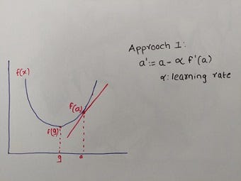
John is skeptical about this approach and doesn’t want to walk more if by chance they end up at the wrong point. So Emily comes up with a new approach:
2. Emily suggests that she will first go to next potential points and calculate the value of the loss function at those points. She keeps a note of the value of the function at all those points, and she will signal John to come to that point where the value is least. John loved this approach as he will never end up at a wrong point. However, poor Emily need to explore all points in her neighborhood and calculate the value of the function at all those points. The beauty of XGBoost is it intelligently tackles both these problems.
Please be advised I may use function/base learner/tree interchangeably.
Gradient Boosting
Many implementations of Gradient Boosting follow approach 1 to minimize the objective function. At every iteration, we fit a base learner to the negative gradient of the loss function and multiply our prediction with a constant and add it to the value from previous iteration.
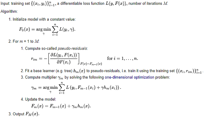
Source: Wikipedia
The intuition is by fitting a base learner to the negative gradient at each iteration is essentially performing gradient descent on the loss function. The negative gradients are often called as pseudo residuals, as they indirectly help us to minimize the objective function.
XGBoost
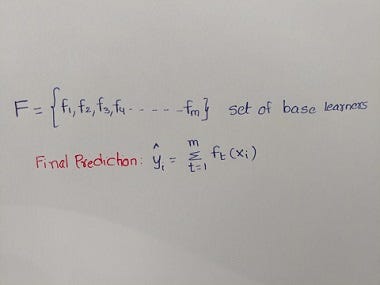
It was a result of research by Tianqi Chen, Ph.D. student at University of Washington. XGBoost is an ensemble additive model that is composed of several base learners.
How should we chose a function at each iteration? we chose a function that minimizes the overall loss.
In the gradient boosting algorithm stated above, we obtained ft(xi) at each iteration by fitting a base learner to the negative gradient of loss function with respect to previous iteration’s value. In XGBoost, we explore several base learners or functions and pick a function that minimizes the loss (Emily’s second approach). As I stated above, there are two problems with this approach:
1. exploring different base learners
2. calculating the value of the loss function for all those base learners.
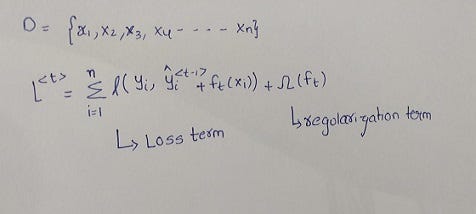
XGBoost uses Taylor series to approximate the value of the loss function for a base learner ft(xi), thus, reducing the load on Emily to calculate the exact loss for different possible base learners.
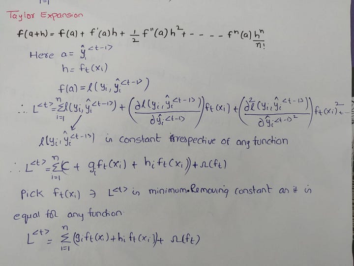
It only uses expansion up to second order derivative assuming this level of approximation would be suffice. The first term ‘C’ is constant irrespective of any ft(xi) we pick. ‘gi’ is the first order derivative of loss at previous iteration with respect predictions at previous iteration. ‘hi’ is the second order derivative of loss at previous iteration with respect to predictions at previous iteration. Therefore, Emily can calculate ‘gi’ and ‘fi’ before starting exploring different base learners, as it will be just a matter of multiplications thereafter. Plug and play, isn’t it?
So XGBoost has reduced one of the burdens on Emily. Still we have a problem of exploring different base learners.
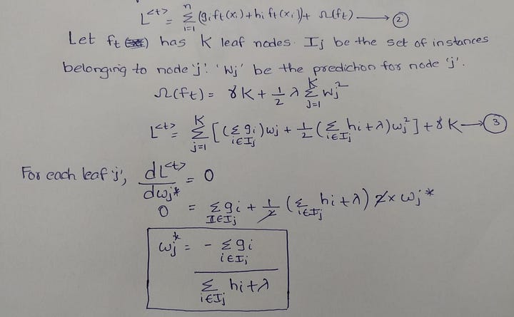
Assume Emily fixed a base learner ft that has ‘K’ leaf nodes. Let Ij be the set of instances belonging to node ‘j’ and ‘wj’ be the prediction for that node. So for an instance ‘i’ belonging to Ij, ft(xi)=wj. Therefore, we obtained equation 3 from equation 2 by substituting ft(xi) with respective predictions. After substituting the predictions, we can take the derivative of loss function with respect to each leaf node’s weight, to get an optimal weight.
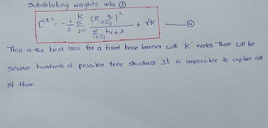
Substituting the optimal weights back into equation 3 gives equation 4. However, this is the optimal loss for a fixed tree structure. There will be several hundreds of possible trees.
Let's formulate the current position of Emily. She now knows how to ease the burden of computing loss using Taylor expansion. She knows for a fixed tree structure what should be the optimal weights in the leaf node. The only thing that is still a concern is how to explore all different possible tree structures.
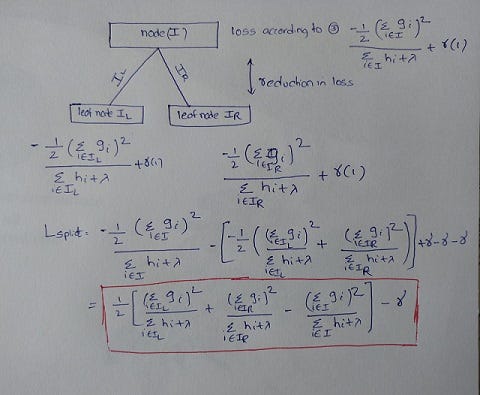
Instead of exploring all possible tree structures, XGBoost greedily builds a tree. The split that results in maximum loss reduction is chosen. In the above picture, the tree starts at Node ‘I’. Based on some split criteria, the node is divided into left and right branches. So some instances fall in left node and other instances fall in right leaf node. Now, we can calculate the reduction in loss and pick the split that causes best reduction in loss.
But still Emily has one more problem. How to chose the split criteria? XGBoost uses different tricks to come up with different split points like histogram, exact, etc. I will not be dealing with that part, as this article has already grown in size.
Bullet Points to Remember
- While Gradient Boosting follows negative gradients to optimize the loss function, XGBoost uses Taylor expansion to calculate the value of the loss function for different base learners. Here is the best video on the internet that explains Taylor expansion.
- XGBoost doesn’t explore all possible tree structures but builds a tree greedily.
- XGBoost’s regularization term penalizes building complex tree with several leaf nodes.
- XGBoost has several other tricks under its sleeve like Column subsampling, shrinkage, splitting criteria, etc. I highly recommend continue reading the original paper here.
You can view the complete derivation here.
Read my other article on PCA here.
Bio: Ajit Samudrala is an aspiring Data Scientist and Data Science intern at SiriusXM.
Original. Reposted with permission.
Related:
- Intuitive Ensemble Learning Guide with Gradient Boosting
- Introduction to Python Ensembles
- CatBoost vs. Light GBM vs. XGBoost