Image by Author

When you’re familiarizing yourself with the unsupervised learning paradigm, you'll learn about clustering algorithms. 

The goal of clustering is often to understand patterns in the given unlabeled dataset. Or it can be to find groups in the dataset—and label them—so that we can perform supervised learning on the now-labeled dataset. This article will cover the basics of hierarchical clustering.

What Is Hierarchical Clustering?

Hierarchical clustering algorithm aims at finding similarity between instances—quantified by a distance metric—to group them into segments called clusters. 

The goal of the algorithm is to find clusters such that data points in a cluster are more similar to each other than they are to data points in other clusters.

There are two common hierarchical clustering algorithms, each with its own approach: 

• Agglomerative Clustering
• Divisive Clustering

Agglomerative Clustering 

Suppose there are n distinct data points in the dataset. Agglomerative clustering works as follows:

1. Start with n clusters; each data point is a cluster in itself.
2. Group data points together based on similarity between them. Meaning similar clusters are merged depending on the distance.
3. Repeat step 2 until there is only one cluster.

Divisive Clustering

As the name suggests, divisive clustering tries to perform the inverse of agglomerative clustering:

1. All the n data points are in a single cluster.
2. Divide this single large cluster into smaller groups. Note that the grouping together of data points in agglomerative clustering is based on similarity. But splitting them into different clusters is based on dissimilarity; data points in different clusters are dissimilar to each other.
3. Repeat until each data point is a cluster in itself.

Distance Metrics

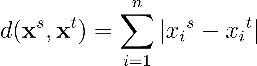
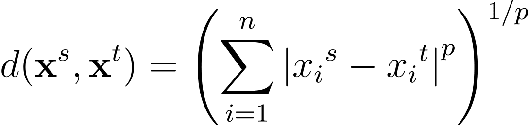
As mentioned, the similarity between data points is quantified using distance. Commonly used distance metrics include the Euclidean and Manhattan distance.

For any two data points in the n-dimensional feature space, the Euclidean distance between them given by:

Another commonly used distance metric is the Manhattan distance given by:

The Minkowski distance is a generalization—for a general p >= 1—of these distance metrics in an n-dimensional space:

Distance Between Clusters: Understanding Linkage Criteria

Using the distance metrics, we can compute the distance between any two data points in the dataset. But you also need to define a distance to determine “how” to group together clusters at each step.

Recall that at each step in agglomerative clustering, we pick the two closest groups to merge. This is captured by the linkage criterion. And the commonly used linkage criteria include:

• Single linkage
• Complete linkage
• Average linkage
• Ward’s linkage

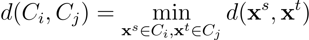
Single Linkage

In single linkage or single-link clustering, the distance between two groups/clusters is taken as the smallest distance between all pairs of data points in the two clusters.
 

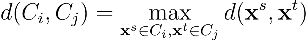
Complete Linkage 

In complete linkage or complete-link clustering, the distance between two clusters is chosen as the largest distance between all pairs of points in the two clusters.

Average Linkage

Sometimes average linkage is used which uses the average of the distances between all pairs of data points in the two clusters.

Ward’s Linkage

Ward's linkage aims to minimize the variance within the merged clusters: merging clusters should minimize the overall increase in variance after merging. This leads to more compact and well-separated clusters.

The distance between two clusters is calculated by considering the increase in the total sum of squared deviations (variance) from the mean of the merged cluster. The idea is to measure how much the variance of the merged cluster increases compared to the variance of the individual clusters before merging.

When we code hierarchical clustering in Python, we’ll use Ward’s linkage, too.

What Is a Dendrogram?

We can visualize the result of clustering as a dendrogram. It is a hierarchical tree structure that helps us understand how the data points—and subsequently clusters—are grouped or merged together as the algorithm proceeds.

In the hierarchical tree structure, the leaves denote the instances or the data points in the data set. The corresponding distances at which the merging or grouping occurs can be inferred from the y-axis.

Sample Dendrogram | Image by Author

Because the type of linkage determines how the data points are grouped together, different linkage criteria yield different dendrograms.

Based on the distance, we can use the dendrogram—cut or slice it at a specific point—to get the required number of clusters.

Unlike some clustering algorithms like K-Means clustering, hierarchical clustering does not require you to specify the number of clusters beforehand. However, agglomerative clustering can be computationally very expensive when working with large datasets. 

Hierarchical Clustering in Python with SciPy

Next, we’ll perform hierarchical clustering on the built-in wine dataset—one step at a time. To do so, we’ll leverage the clustering package—scipy.cluster—from SciPy.

Step 1 – Import Necessary Libraries

First, let's import the libraries and the necessary modules from the libraries scikit-learn and SciPy:

# imports
import pandas as pd
import matplotlib.pyplot as plt
from sklearn.datasets import load_wine
from sklearn.preprocessing import MinMaxScaler
from scipy.cluster.hierarchy import dendrogram, linkage

Step 2 – Load and Preprocess the Dataset

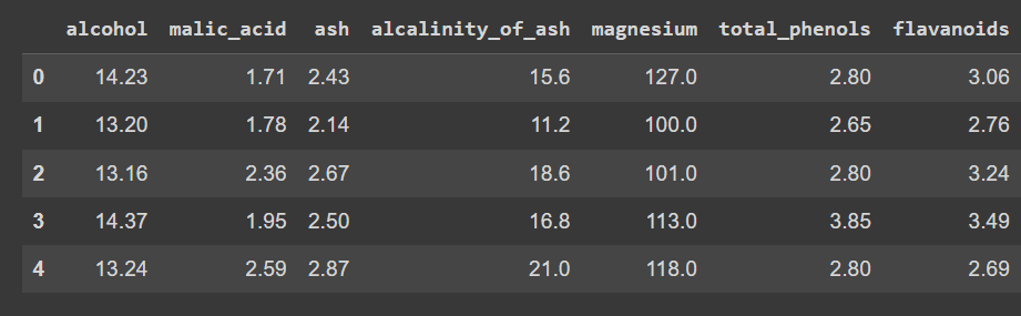
Next, we load the wine dataset into a pandas dataframe. It is a simple dataset that is part of scikit-learn’s datasets and is helpful in exploring hierarchical clustering.

# Load the dataset
data = load_wine()
X = data.data

# Convert to DataFrame
wine_df = pd.DataFrame(X, columns=data.feature_names)

Let’s check the first few rows of the dataframe:

wine_df.head()

Truncated output of wine_df.head()

Notice that we’ve loaded only the features—and not the output label—so that we can peform clustering to discover groups in the dataset. 

Let's check the shape of the dataframe:

print(wine_df.shape)

There are 178 records and 14 features:

Output >>> (178, 14)

Because the data set contains numeric values that are spread across different ranges, let's preprocess the dataset. We’ll use MinMaxScaler to transform each of the features to take on values in the range [0, 1].

# Scale the features using MinMaxScaler
scaler = MinMaxScaler()
X_scaled = scaler.fit_transform(X)

Step 3 – Perform Hierarchical Clustering and Plot the Dendrogram

Let’s compute the linkage matrix, perform clustering, and plot the dendrogram. We can use linkage from the hierarchy module to calculate the linkage matrix based on Ward’s linkage (set method to 'ward').

As discussed, Ward’s linkage minimizes the variance within each cluster. We then plot the dendrogram to visualize the hierarchical clustering process.

# Calculate linkage matrix
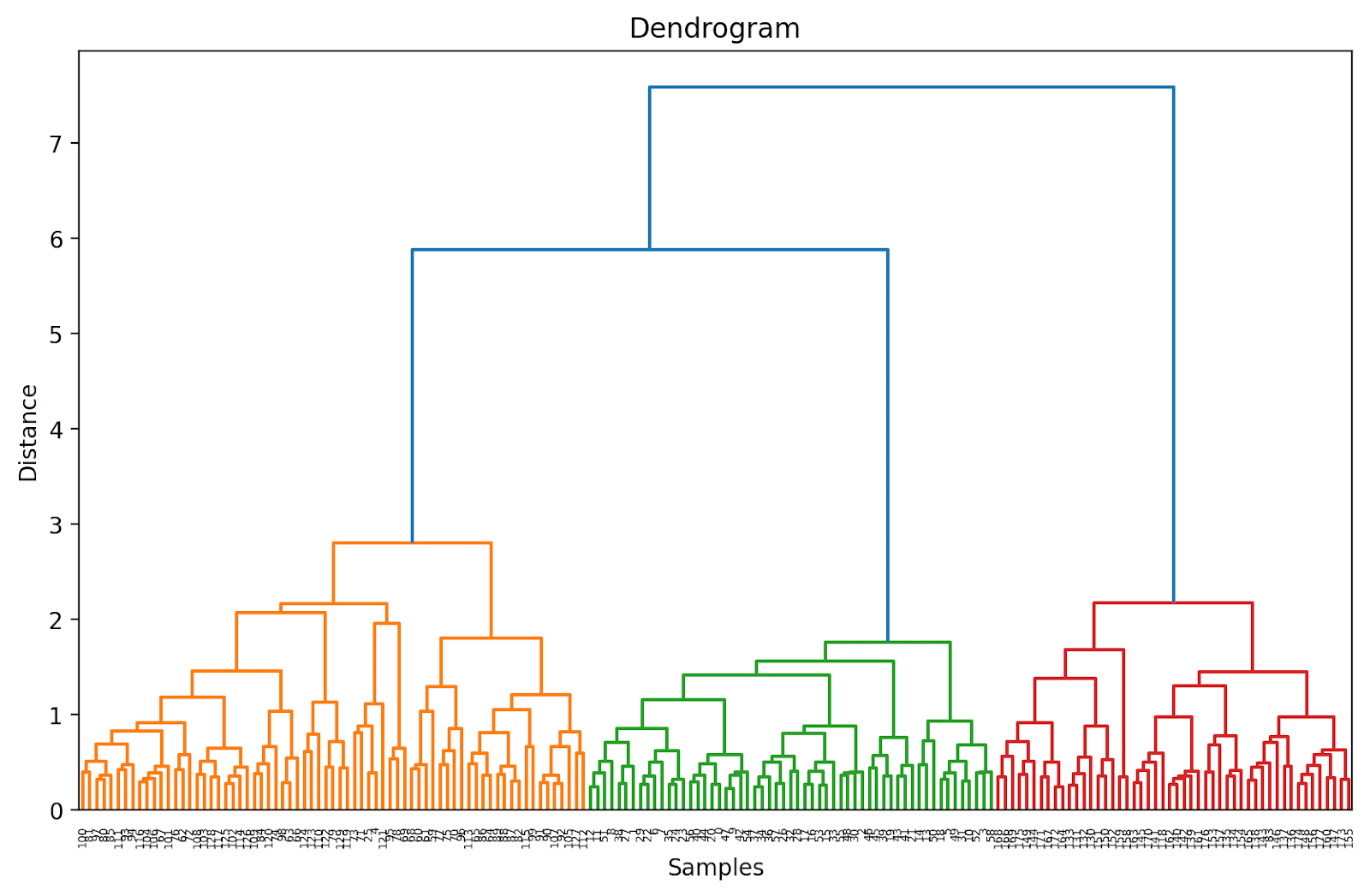
linked = linkage(X_scaled, method='ward')

# Plot dendrogram
plt.figure(figsize=(10, 6),dpi=200)
dendrogram(linked, orientation='top', distance_sort='descending', show_leaf_counts=True)
plt.title('Dendrogram')
plt.xlabel('Samples')
plt.ylabel('Distance')
plt.show()

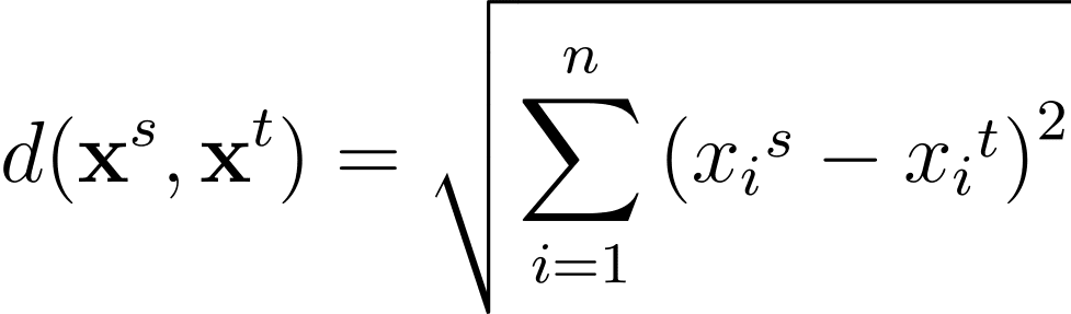
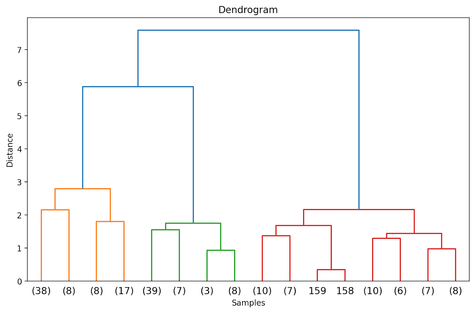
Because we haven't (yet) truncated the dendrogram, we get to visualize how each of the 178 data points are grouped together into a single cluster. Though this is seemingly difficult to interpret, we can still see that there are three different clusters.

Truncating the Dendrogram for Easier Visualization

In practice, instead of the entire dendrogram, we can visualize a truncated version that's easier to interpret and understand.

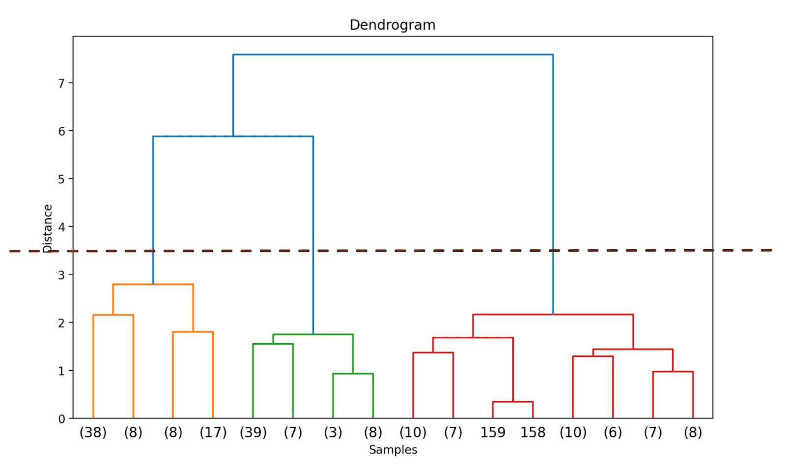
To truncate the dendrogram, we can set truncate_mode to 'level' and p = 3. 

# Calculate linkage matrix
linked = linkage(X_scaled, method='ward')

# Plot dendrogram
plt.figure(figsize=(10, 6),dpi=200)
dendrogram(linked, orientation='top', distance_sort='descending', truncate_mode='level', p=3, show_leaf_counts=True)
plt.title('Dendrogram')
plt.xlabel('Samples')
plt.ylabel('Distance')
plt.show()

Doing so will truncate the dendrogram to include only those clusters which are within 3 levels from the final merge.

In the above dendrogram, you can see that some data points such as 158 and 159 are represented individually. Whereas some others are mentioned within parentheses; these are not individual data points but the number of data points in a cluster. (k) denotes a cluster with k samples.

Step 4 – Identify the Optimal Number of Clusters

The dendrogram helps us choose the optimal number of clusters. 

We can observe where the distance along the y-axis increases drastically, choose to truncate the dendrogram at that point—and use the distance as the threshold to form clusters. 

For this example, the optimal number of clusters is 3.

Step 5 – Form the Clusters 

Once we have decided on the optimal number of clusters, we can use the corresponding distance along the y-axis—a threshold distance. This ensures that above the threshold distance, the clusters are no longer merged. We choose a threshold_distance of 3.5 (as inferred from the dendrogram).

We then use fcluster with criterion set to 'distance' to get the cluster assignment for all the data points:

from scipy.cluster.hierarchy import fcluster

# Choose a threshold distance based on the dendrogram
threshold_distance = 3.5  

# Cut the dendrogram to get cluster labels
cluster_labels = fcluster(linked, threshold_distance, criterion='distance')

# Assign cluster labels to the DataFrame
wine_df['cluster'] = cluster_labels

You should now be able to see the cluster labels (one of {1, 2, 3}) for all the data points:

print(wine_df['cluster'])

Output >>>
0      2
1      2
2      2
3      2
4      3
      ..
173    1
174    1
175    1
176    1
177    1
Name: cluster, Length: 178, dtype: int32

Step 6 – Visualize the Clusters

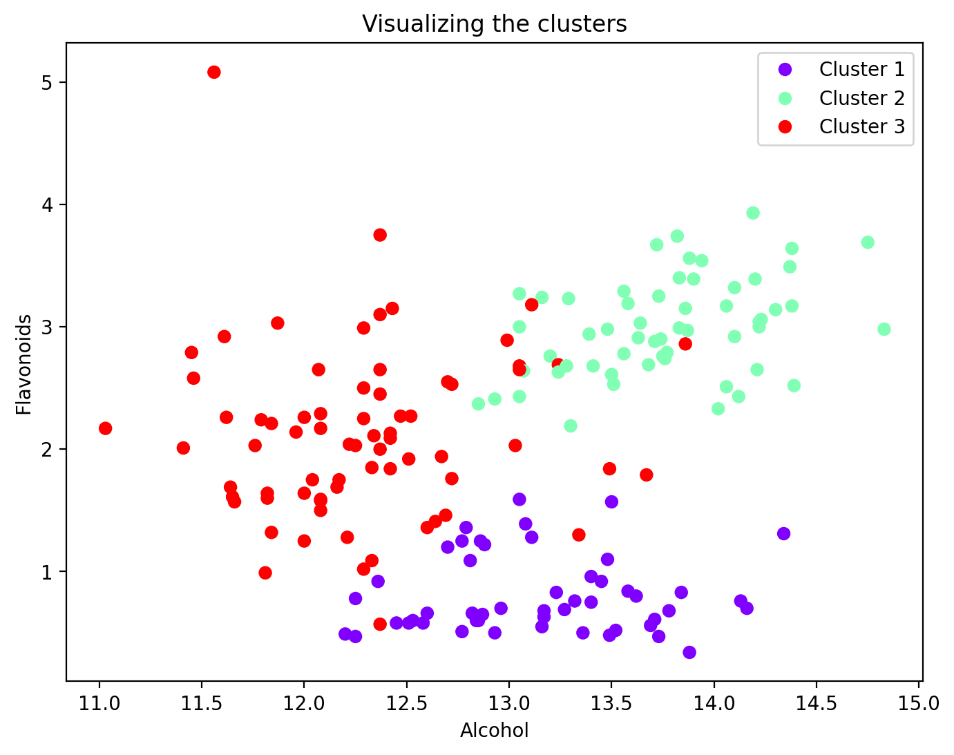
Now that each data point has been assigned to a cluster, you can visualize a subset of features and their cluster assignments. Here's the scatter plot of two such features along with their cluster mapping:

plt.figure(figsize=(8, 6))

scatter = plt.scatter(wine_df['alcohol'], wine_df['flavanoids'], c=wine_df['cluster'], cmap='rainbow')
plt.xlabel('Alcohol')
plt.ylabel('Flavonoids')
plt.title('Visualizing the clusters')

# Add legend
legend_labels = [f'Cluster {i + 1}' for i in range(n_clusters)]
plt.legend(handles=scatter.legend_elements()[0], labels=legend_labels)

plt.show()

Wrapping Up

And that's a wrap! In this tutorial, we used SciPy to perform hierarchical clustering just so we can cover the steps involved in greater detail. Alternatively, you can also use the AgglomerativeClustering class from scikit-learn’s cluster module. Happy coding clustering!

References

[1] Introduction to Machine Learning

[2] An Introduction to Statistical Learning (ISLR)
 
 
Bala Priya C is a developer and technical writer from India. She likes working at the intersection of math, programming, data science, and content creation. Her areas of interest and expertise include DevOps, data science, and natural language processing. She enjoys reading, writing, coding, and coffee! Currently, she's working on learning and sharing her knowledge with the developer community by authoring tutorials, how-to guides, opinion pieces, and more.