Introduction to Clustering in Python with PyCaret
A step-by-step, beginner-friendly tutorial for unsupervised clustering tasks in Python using PyCaret.
By Moez Ali, Founder & Author of PyCaret
Photo by Paola Galimberti on Unsplash
1. Introduction
PyCaret is an open-source, low-code machine learning library in Python that automates machine learning workflows. It is an end-to-end machine learning and model management tool that speeds up the experiment cycle exponentially and makes you more productive.
In comparison with the other open-source machine learning libraries, PyCaret is an alternate low-code library that can be used to replace hundreds of lines of code with few lines only. This makes experiments exponentially fast and efficient. PyCaret is essentially a Python wrapper around several machine learning libraries and frameworks such as scikit-learn, XGBoost, LightGBM, CatBoost, spaCy, Optuna, Hyperopt, Ray, and a few more.
The design and simplicity of PyCaret are inspired by the emerging role of citizen data scientists, a term first used by Gartner. Citizen Data Scientists are power users who can perform both simple and moderately sophisticated analytical tasks that would previously have required more technical expertise.
To learn more about PyCaret, you can check the official website or GitHub.
2. Tutorial Objective
In this tutorial we will learn:
- Getting Data: How to import data from the PyCaret repository.
- Set up Environment: How to set up an experiment in PyCaret’s unsupervised clustering module.
- Create Model: How to train unsupervised clustering models and assign cluster labels to the training dataset for further analysis.
- Plot Model: How to analyze model performance using various plots (Elbow, Silhouette, Distribution, etc.).
- Predict Model: How to assign cluster labels to new and unseen datasets based on a trained model.
- Save/Load Model: How to save/load model for future use.
3. Installing PyCaret
Installation is easy and will only take a few minutes. PyCaret’s default installation from pip only installs hard dependencies as listed in the requirements.txt file.
pip install pycaret
To install the full version:
pip install pycaret[full]
4. What is Clustering?
Clustering is the task of grouping a set of objects in such a way that those in the same group (called a cluster) are more similar to each other than to those in other groups. It is an exploratory data mining activity, and a common technique for statistical data analysis used in many fields including machine learning, pattern recognition, image analysis, information retrieval, bioinformatics, data compression, and computer graphics. Some common real-life use cases of clustering are:
- Customer segmentation based on purchase history or interests to design targeted marketing campaigns.
- Cluster documents into multiple categories based on tags, topics, and the content of the document.
- Analysis of outcome in social / life science experiments to find natural groupings and patterns in the data.
5. Overview of Clustering Module in PyCaret
PyCaret’s clustering module (pycaret.clustering) is an unsupervised machine learning module that performs the task of grouping a set of objects in such a way that those in the same group (called a cluster) are more similar to each other than to those in other groups.
PyCaret’s clustering module provides several pre-processing features that can be configured when initializing the setup through the setup function. It has over 8 algorithms and several plots to analyze the results. PyCaret's clustering module also implements a unique function called tune_model that allows you to tune the hyperparameters of a clustering model to optimize a supervised learning objective such as AUC for classification or R2 for regression.
6. Dataset for the Tutorial
In this tutorial, we will use a dataset from UCI called Mice Protein Expression. The data set consists of the expression levels of 77 proteins that produced detectable signals in the nuclear fraction of the cortex. The dataset contains a total of 1080 measurements per protein. Each measurement can be considered as an independent sample (mouse).
Dataset Citation:
Higuera C, Gardiner KJ, Cios KJ (2015) Self-Organizing Feature Maps Identify Proteins Critical to Learning in a Mouse Model of Down Syndrome. PLoS ONE 10(6): e0129126. [Web Link] journal.pone.0129126
You can download the data from the original source found here and load it using pandas (Learn How) or you can use PyCaret’s data repository to load the data using the get_data() function (This will require an internet connection).
from pycaret.datasets import get_data
dataset = get_data('mice')
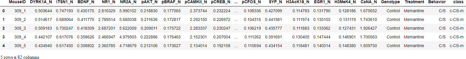
# check the shape of data
dataset.shape>>> (1080, 82)
In order to demonstrate the use of the predict_model function on unseen data, a sample of 5% (54 records) has been withheld from the original dataset to be used for predictions at the end of the experiment.
data = dataset.sample(frac=0.95, random_state=786)
data_unseen = dataset.drop(data.index)

data.reset_index(drop=True, inplace=True)
data_unseen.reset_index(drop=True, inplace=True)

print('Data for Modeling: ' + str(data.shape))
print('Unseen Data For Predictions: ' + str(data_unseen.shape))>>> Data for Modeling: (1026, 82)
>>> Unseen Data For Predictions: (54, 82)
8. Setting up Environment in PyCaret
The setup function in PyCaret initializes the environment and creates the transformation pipeline for modeling and deployment. setup must be called before executing any other function in pycaret. It takes only one mandatory parameter: a pandas dataframe. All other parameters are optional can be used to customize the preprocessing pipeline.
When setup is executed, PyCaret's inference algorithm will automatically infer the data types for all features based on certain properties. The data type should be inferred correctly but this is not always the case. To handle this, PyCaret displays a prompt, asking for data types confirmation, once you execute the setup. You can press enter if all data types are correct or type quit to exit the setup.
Ensuring that the data types are correct is really important in PyCaret as it automatically performs multiple type-specific preprocessing tasks which are imperative for machine learning models.
Alternatively, you can also use numeric_features and categorical_features parameters in the setup to pre-define the data types.
from pycaret.clustering import *

exp_clu101 = setup(data, normalize = True,
                   ignore_features = ['MouseID'],
                   session_id = 123)
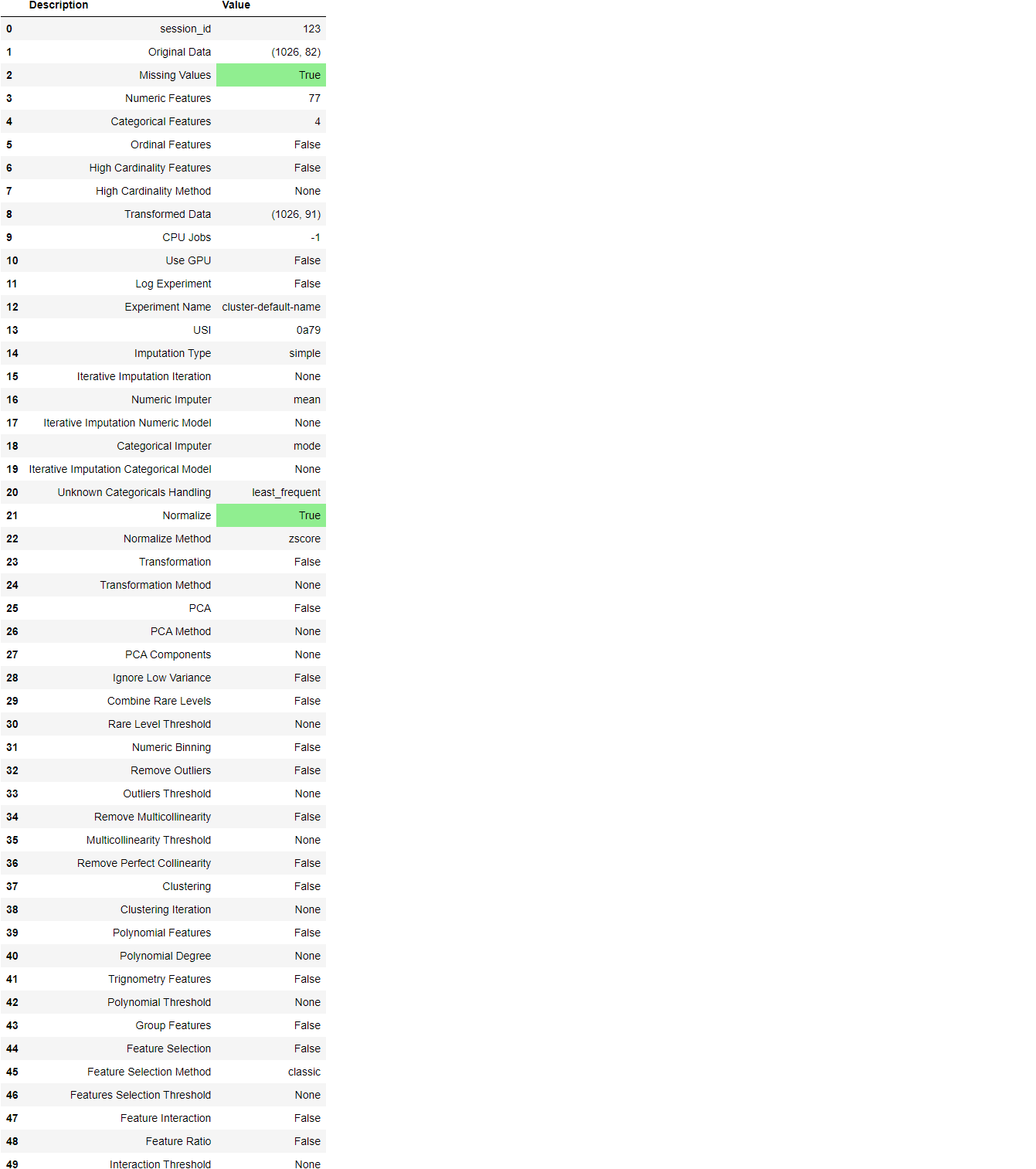
Once the setup has been successfully executed it displays the information grid which contains some important information about the experiment. Most of the information is related to the pre-processing pipeline which is constructed when setup is executed. The majority of these features are out of scope for this tutorial, however, a few important things to note are:
- session_id: A pseduo-random number distributed as a seed in all functions for later reproducibility. If no
session_idis passed, a random number is automatically generated that is distributed to all functions. In this experiment, thesession_idis set as123for later reproducibility. - Missing Values: When there are missing values in original data this will show as True. Notice that
Missing Valuesin the information grid above isTrueas the data contains missing values which are automatically imputed usingmeanfor the numeric features andconstantfor the categorical features in the dataset. The method of imputation can be changed using thenumeric_imputationandcategorical_imputationparameters in thesetupfunction. - Original Data: Displays the original shape of the dataset. In this experiment (1026, 82) means 1026 samples and 82 features.
- Transformed Data: Displays the shape of the transformed dataset. Notice that the shape of the original dataset (1026, 82) is transformed into (1026, 91). The number of features has increased due to the encoding of categorical features in the dataset.
- Numeric Features: The number of features inferred as numeric. In this dataset, 77 out of 82 features are inferred as numeric.
- Categorical Features: The number of features inferred as categorical. In this dataset, 5 out of 82 features are inferred as categorical. Also notice that we have ignored one categorical feature
MouseIDusing theignore_featureparameter since it's a unique identifier for each sample and we don’t want it to be considered during model training.
Notice how a few tasks that are imperative to perform modeling are automatically handled such as missing value imputation, categorical encoding, etc. Most of the parameters in the setup function are optional and used for customizing the pre-processing pipeline. These parameters are out of scope for this tutorial but I will write more about them later.
9. Create a Model
Training a clustering model in PyCaret is simple and similar to how you would create a model in the supervised learning modules of PyCaret. A clustering model is created using the create_model function. This function returns a trained model object and a few unsupervised metrics. See an example below:
kmeans = create_model('kmeans')

print(kmeans)>>> OUTPUT
KMeans(algorithm='auto', copy_x=True, init='k-means++', max_iter=300,
       n_clusters=4, n_init=10, n_jobs=-1, precompute_distances='deprecated',
       random_state=123, tol=0.0001, verbose=0)
We have trained an unsupervised K-Means model using the create_model. Notice the n_clusters parameter is set to 4 which is the default when you do not pass a value to the num_clusters parameter. In the below example we will create a kmodes model with 6 clusters.
kmodes = create_model('kmodes', num_clusters = 6)

print(kmodes)>>> OUTPUT
KModes(cat_dissim=<function matching_dissim at 0x00000168B0B403A0>, init='Cao',
       max_iter=100, n_clusters=6, n_init=1, n_jobs=-1, random_state=123,
       verbose=0)
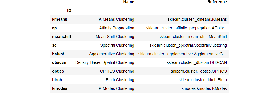
To see the complete list of models available in the model library, please check the documentation or use the models function.
models()
10. Assign a Model
Now that we have trained a model, we can assign the cluster labels to our training dataset (1026 samples) by using the assign_model function.
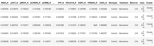
kmean_results = assign_model(kmeans)
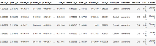
kmean_results.head()
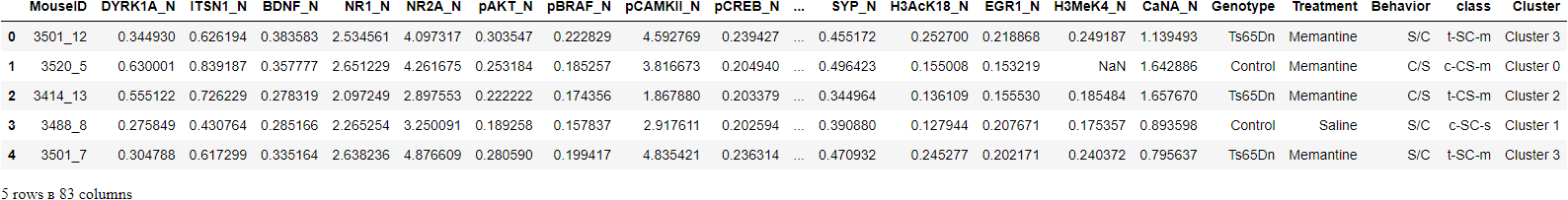
Notice that a new column called Cluster has been added to the original dataset.
Note that the results also include the MouseID column that we actually dropped during the setup. Don’t worry, it is not used for the model training, rather is only appended to the dataset only when assign_model is called.
11. Plot a Model
The plot_model function is used to analyze clustering models. This function takes a trained model object and returns a plot.
11.1 Cluster PCA Plot
plot_model(kmeans)
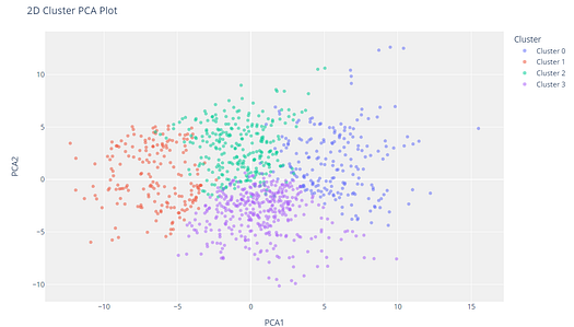
The cluster labels are automatically colored and shown in a legend. When you hover over the data points you will see additional features which by default use the first column of the dataset (in this case MouseID). You can change this by passing the feature parameter and you may also set label to True if you want labels to be printed on the plot.
11.2 Elbow Plot
plot_model(kmeans, plot = 'elbow')
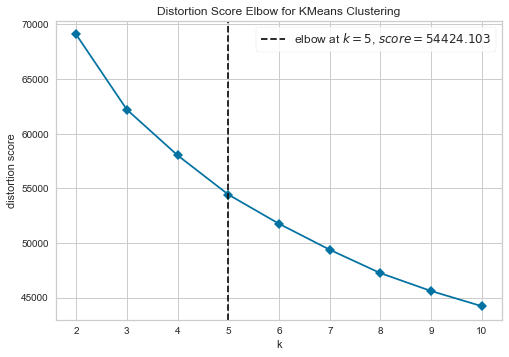
The elbow method is a heuristic method of interpretation and validation of consistency within-cluster analysis designed to help find the appropriate number of clusters in a dataset. In this example, the Elbow plot above suggests that 5 is the optimal number of clusters.
11.3 Silhouette Plot
plot_model(kmeans, plot = 'silhouette')
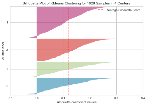
Silhouette is a method of interpretation and validation of consistency within clusters of data. The technique provides a succinct graphical representation of how well each object has been classified. In other words, the silhouette value is a measure of how similar an object is to its own cluster (cohesion) compared to other clusters (separation).
Learn More about Silhouette Plot
11.4 Distribution Plot
plot_model(kmeans, plot = 'distribution')
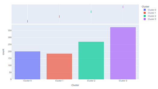
The distribution plot shows the size of each cluster. When hovering over the bars you will see the number of samples assigned to each cluster. From the example above, we can observe that cluster 3 has the highest number of samples. We can also use the distribution plot to see the distribution of cluster labels in association with any other numeric or categorical feature.
plot_model(kmeans, plot = 'distribution', feature = 'class')
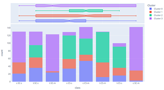
In the above example, we have used the class as a feature so each bar represents a class which is colored with a cluster label (legend on right). We can observe that class t-SC-m and c-SC-m are mostly dominated by Cluster 3. We can also use the same plot to see the distribution of any continuous feature.
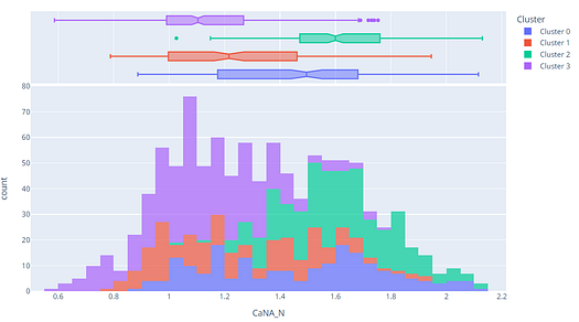
plot_model(kmeans, plot = 'distribution', feature = 'CaNA_N')
12. Predict on unseen data
The predict_model function is used to assign cluster labels to a new unseen dataset. We will now use our trained kmeans model to predict the data stored in data_unseen. This variable was created at the beginning of the tutorial and contains 54 samples from the original dataset that were never exposed to PyCaret.
unseen_predictions = predict_model(kmeans, data=data_unseen)
unseen_predictions.head()
13. Saving the model
We have now finished the experiment by using our kmeans model to predict labels on unseen data.
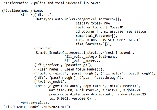
This brings us to the end of our experiment, but one question is still to be asked: What happens when you have more new data to predict? Do you have to go through the entire experiment again? The answer is no, PyCaret’s inbuilt function save_model allows you to save the model along with the entire transformation pipeline for later use.
save_model(kmeans,’Final KMeans Model 25Nov2020')
To load a saved model at a future date in the same or an alternative environment, we would use PyCaret’s load_model function and then easily apply the saved model on new unseen data for prediction.
saved_kmeans = load_model('Final KMeans Model 25Nov2020')
new_prediction = predict_model(saved_kmeans, data=data_unseen)
new_prediction.head()
14. Wrap-up / Next Steps?
We have only covered the basics of PyCaret’s clustering module. In the following tutorials, we will go deeper into advanced pre-processing techniques that allow you to fully customize your machine learning pipeline and are a must-know for any data scientist.
Thank you for reading ????
Important Links
⭐ Tutorials New to PyCaret? Check out our official notebooks!
???? Example Notebooks created by the community.
???? Blog Tutorials and articles by contributors.
???? Documentation The detailed API docs of PyCaret
???? Video Tutorials Our video tutorial from various events.
???? Discussions Have questions? Engage with community and contributors.
????️ Changelog Changes and version history.
???? Roadmap PyCaret’s software and community development plan.
Bio: Moez Ali writes about PyCaret and its use-cases in the real world, If you would like to be notified automatically, you can follow Moez on Medium, LinkedIn, and Twitter.
Original. Reposted with permission.
Related: