Introduction to Binary Classification with PyCaret

PyCaret is an alternate low-code library that can be used to replace hundreds of lines of code with few lines only. See how to use it for binary classification.

comments

By Moez Ali, Founder & Author of PyCaret

Photo by Mike U on Unsplash

1.0 Introduction

PyCaret is an open-source, low-code machine learning library in Python that automates machine learning workflows. It is an end-to-end machine learning and model management tool that speeds up the experiment cycle exponentially and makes you more productive.

In comparison with the other open-source machine learning libraries, PyCaret is an alternate low-code library that can be used to replace hundreds of lines of code with few lines only. This makes experiments exponentially fast and efficient. PyCaret is essentially a Python wrapper around several machine learning libraries and frameworks such as scikit-learn, XGBoost, LightGBM, CatBoost, spaCy, Optuna, Hyperopt, Ray, and a few more.

The design and simplicity of PyCaret are inspired by the emerging role of citizen data scientists, a term first used by Gartner. Citizen Data Scientists are power users who can perform both simple and moderately sophisticated analytical tasks that would previously have required more technical expertise.

To learn more about PyCaret, you can check the official website or GitHub.

2.0 Tutorial Objective

In this tutorial we will learn:

Getting Data: How to import data from the PyCaret repository
Setting up Environment: How to set up an experiment in PyCaret and get started with building classification models
Create Model: How to create a model, perform stratified cross-validation and evaluate classification metrics
Tune Model: How to automatically tune the hyper-parameters of a classification model
Plot Model: How to analyze model performance using various plots
Finalize Model: How to finalize the best model at the end of the experiment
Predict Model: How to make predictions on unseen data
Save / Load Model: How to save/load a model for future use

3.0 Installing PyCaret

Installation is easy and will only take a few minutes. PyCaret’s default installation from pip only installs hard dependencies as listed in the requirements.txt file.

pip install pycaret

To install the full version:

pip install pycaret[full]

4.0 What is Binary Classification?

Binary classification is a supervised machine learning technique where the goal is to predict categorical class labels which are discrete and unordered such as Pass/Fail, Positive/Negative, Default/Not-Default, etc. A few real-world use cases for classification are listed below:

Medical testing to determine if a patient has a certain disease or not — the classification property is the presence of the disease.
A “pass or fail” test method or quality control in factories, i.e. deciding if a specification has or has not been met — a go/no-go classification.
Information retrieval, namely deciding whether a page or an article should be in the result set of a search or not — the classification property is the relevance of the article or the usefulness to the user.

5.0 Overview of the Classification Module in PyCaret

PyCaret’s classification module (pycaret.classification) is a supervised machine learning module that is used for classifying the elements into a binary group based on various techniques and algorithms. Some common use cases of classification problems include predicting customer default (yes or no), customer churn (customer will leave or stay), disease found (positive or negative).

The PyCaret classification module can be used for Binary or Multi-class classification problems. It has over 18 algorithms and 14 plots to analyze the performance of models. Be it hyper-parameter tuning, ensembling, or advanced techniques like stacking, PyCaret’s classification module has it all.

6.0 Dataset for the Tutorial

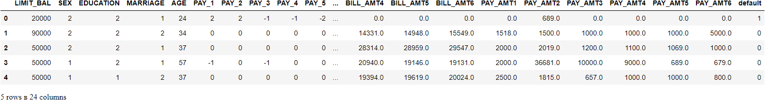
For this tutorial, we will use a dataset from UCI called Default of Credit Card Clients Dataset. This dataset contains information on default payments, demographic factors, credit data, payment history, and billing statements of credit card clients in Taiwan from April 2005 to September 2005. There are 24,000 samples and 25 features. Short descriptions of each column are as follows:

ID: ID of each client
LIMIT_BAL: Amount of given credit in NT dollars (includes individual and family/supplementary credit)
SEX: Gender (1=male, 2=female)
EDUCATION: (1=graduate school, 2=university, 3=high school, 4=others, 5=unknown, 6=unknown)
MARRIAGE: Marital status (1=married, 2=single, 3=others)
AGE: Age in years
PAY_0 to PAY_6: Repayment status by n months ago (PAY_0 = last month … PAY_6 = 6 months ago) (Labels: -1=pay duly, 1=payment delay for one month, 2=payment delay for two months, … 8=payment delay for eight months, 9=payment delay for nine months and above)
BILL_AMT1 to BILL_AMT6: Amount of bill statement by n months ago ( BILL_AMT1 = last_month .. BILL_AMT6 = 6 months ago)
PAY_AMT1 to PAY_AMT6: Amount of payment by n months ago ( BILL_AMT1 = last_month .. BILL_AMT6 = 6 months ago)
default: Default payment (1=yes, 0=no) Target Column

Dataset Acknowledgement:

Lichman, M. (2013). UCI Machine Learning Repository. Irvine, CA: University of California, School of Information and Computer Science.

7.0 Getting the Data

You can download the data from the original source found here and load it using pandas (learn how) or you can use PyCaret’s data repository to load the data using the get_data() function (This will require an internet connection).

# loading the dataset
from pycaret.datasets import get_data
dataset = get_data('credit')

# check the shape of data
dataset.shape>>> (24000, 24)

In order to demonstrate the use of the predict_model function on unseen data, a sample of 1200 records (~5%) has been withheld from the original dataset to be used for predictions at the end. This should not be confused with a train-test-split, as this particular split is performed to simulate a real-life scenario. Another way to think about this is that these 1200 customers are not available at the time of training of machine learning models.

# sample 5% of data to be used as unseen data
data = dataset.sample(frac=0.95, random_state=786)
data_unseen = dataset.drop(data.index)
data.reset_index(inplace=True, drop=True)
data_unseen.reset_index(inplace=True, drop=True)# print the revised shape
print('Data for Modeling: ' + str(data.shape))
print('Unseen Data For Predictions: ' + str(data_unseen.shape))>>> Data for Modeling: (22800, 24)
>>> Unseen Data For Predictions: (1200, 24)

8.0 Setting up Environment in PyCaret

The setup function in PyCaret initializes the environment and creates the transformation pipeline for modeling and deployment. setup must be called before executing any other function in pycaret. It takes two mandatory parameters: a pandas dataframe and the name of the target column. All other parameters are optional can be used to customize the preprocessing pipeline.

When setup is executed, PyCaret's inference algorithm will automatically infer the data types for all features based on certain properties. The data type should be inferred correctly but this is not always the case. To handle this, PyCaret displays a prompt, asking for data types confirmation, once you execute the setup. You can press enter if all data types are correct or type quit to exit the setup.

Ensuring that the data types are correct is really important in PyCaret as it automatically performs multiple type-specific preprocessing tasks which are imperative for machine learning models.

Alternatively, you can also use numeric_features and categorical_features parameters in the setup to pre-define the data types.

# init setup
from pycaret.classification import *
s = setup(data = data, target = 'default', session_id=123)

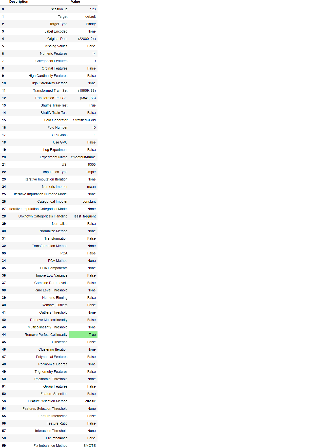
Once the setup has been successfully executed it displays the information grid which contains some important information about the experiment. Most of the information is related to the pre-processing pipeline which is constructed when setup is executed. The majority of these features are out of scope for this tutorial, however, a few important things to note are:

session_id: A pseudo-random number distributed as a seed in all functions for later reproducibility. If no session_id is passed, a random number is automatically generated that is distributed to all functions. In this experiment, the session_id is set as 123 for later reproducibility.
Target Type: Binary or Multiclass. The Target type is automatically detected and shown. There is no difference in how the experiment is performed for Binary or Multiclass problems. All functionalities are identical.
Label Encoded: When the Target variable is of type string (i.e. ‘Yes’ or ‘No’) instead of 1 or 0, it automatically encodes the label into 1 and 0 and displays the mapping (0: No, 1: Yes) for reference. In this experiment, no label encoding is required since the target variable is of type numeric.
Original Data: Displays the original shape of the dataset. In this experiment (22800, 24) means 22,800 samples and 24 features including the target column.
Missing Values: When there are missing values in the original data this will show as True. For this experiment, there are no missing values in the dataset.
Numeric Features: The number of features inferred as numeric. In this dataset, 14 out of 24 features are inferred as numeric.
Categorical Features: The number of features inferred as categorical. In this dataset, 9 out of 24 features are inferred as categorical.
Transformed Train Set: Displays the shape of the transformed training set. Notice that the original shape of (22800, 24) is transformed into (15959, 91) for the transformed train set and the number of features has increased to 91 from 24 due to one-hot-encoding.
Transformed Test Set: Displays the shape of the transformed test/hold-out set. There are 6841 samples in the test/hold-out set. This split is based on the default value of 70/30 that can be changed using the train_size parameter in the setup.

Notice how a few tasks that are imperative to perform modeling are automatically handled such as missing value imputation (in this case there are no missing values in the training data, but we still need imputers for unseen data), categorical encoding, etc. Most of the parameters in the setup are optional and used for customizing the pre-processing pipeline. These parameters are out of scope for this tutorial but we will cover them in future tutorials.

9.0 Comparing All Models

Comparing all models to evaluate performance is the recommended starting point for modeling once the setup is completed (unless you exactly know what kind of model you need, which is often not the case). This function trains all models in the model library and scores them using stratified cross-validation for metric evaluation. The output prints a scoring grid that shows average Accuracy, AUC, Recall, Precision, F1, Kappa, and MCC across the folds (10 by default) along with training times.

best_model = compare_models()

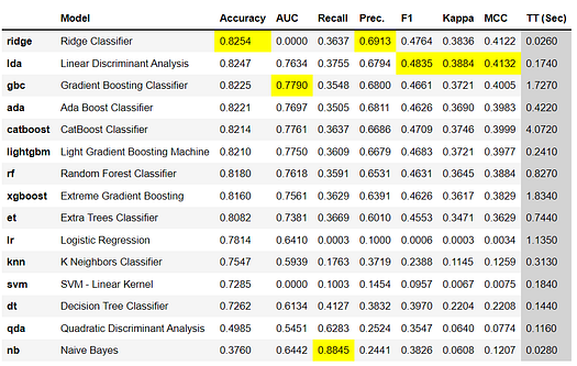
The scoring grid printed above highlights the highest performing metric for comparison purposes only. The grid by default is sorted using Accuracy (highest to lowest) which can be changed by passing the sort parameter. For example compare_models(sort = 'Recall') will sort the grid by recall instead of accuracy.

If you want to change the fold parameter from the default value of 10 to a different value then you can use the fold parameter. For example compare_models(fold = 5) will compare all models on 5 fold cross-validation. Reducing the number of folds will improve the training time. By default, compare_models return the best performing model based on default sort order but can be used to return a list of top N models by using n_select parameter.

print(best_model)>>> OUTPUTRidgeClassifier(alpha=1.0, class_weight=None, copy_X=True, fit_intercept=True,
                max_iter=None, normalize=False, random_state=123, solver='auto',
                tol=0.001)

10.0 Create a Model

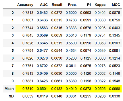
create_model is the most granular function in PyCaret and is often the foundation behind most of the PyCaret functionalities. As the name suggests this function trains and evaluates a model using cross-validation that can be set with fold parameter. The output prints a scoring grid that shows Accuracy, AUC, Recall, Precision, F1, Kappa, and MCC by fold.

For the remaining part of this tutorial, we will work with the below models as our candidate models. The selections are for illustration purposes only and do not necessarily mean they are the top-performing or ideal for this type of data.

Decision Tree Classifier (‘dt’)
K Neighbors Classifier (‘knn’)
Random Forest Classifier (‘rf’)

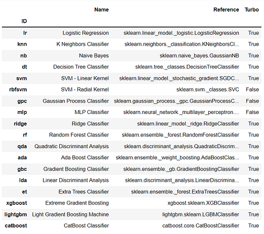
There are 18 classifiers available in the model library of PyCaret. To see a list of all classifiers either check the documentation or use models function to see the library.

# check available models
models()

10.1 Decision Tree Classifier

dt = create_model('dt')

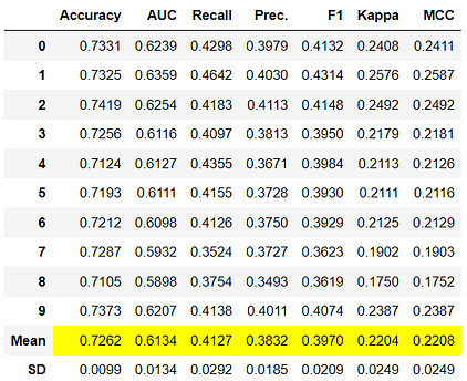
# trained model object is stored in the variable 'dt'. 
print(dt)>>> OUTPUTDecisionTreeClassifier(ccp_alpha=0.0, class_weight=None, criterion='gini',
                       max_depth=None, max_features=None, max_leaf_nodes=None,
                       min_impurity_decrease=0.0, min_impurity_split=None,
                       min_samples_leaf=1, min_samples_split=2,
                       min_weight_fraction_leaf=0.0, presort='deprecated',
                       random_state=123, splitter='best')

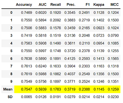
10.2 K Neighbors Classifier

knn = create_model('knn')

10.3 Random Forest Classifier

rf = create_model('rf')

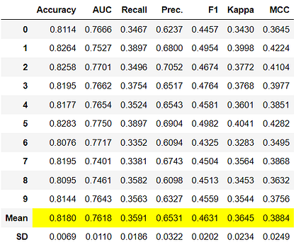
Notice that the mean score of all models matches with the score printed in compare_models. This is because the metrics printed in the compare_models score grid are the average scores across all CV folds. Similar to thecompare_models, if you want to change the fold parameter from the default value of 10 to a different value then you can use the fold parameter. For Example: create_model('dt', fold = 5) will create a Decision Tree Classifier using 5 fold stratified CV.

11.0 Tune a Model

When a model is created using the create_model function it uses the default hyperparameters to train the model. In order to tune hyperparameters, the tune_model function is used. This function automatically tunes the hyperparameters of a model using random grid search on a pre-defined search space. The output prints a scoring grid that shows Accuracy, AUC, Recall, Precision, F1, Kappa, and MCC by fold for the best model. To use the custom search grid, you can pass custom_grid parameter in the tune_model function (see 11.2 KNN tuning below).

11.1 Decision Tree Classifier

tuned_dt = tune_model(dt)

# tuned model object is stored in the variable 'tuned_dt'. 
print(tuned_dt)>>> OUTPUTDecisionTreeClassifier(ccp_alpha=0.0, class_weight=None, criterion='entropy',
                       max_depth=6, max_features=1.0, max_leaf_nodes=None,
                       min_impurity_decrease=0.002, min_impurity_split=None,
                       min_samples_leaf=5, min_samples_split=5,
                       min_weight_fraction_leaf=0.0, presort='deprecated',
                       random_state=123, splitter='best')

11.2 K Neighbors Classifier

import numpy as np
tuned_knn = tune_model(knn, custom_grid = {'n_neighbors' : np.arange(0,50,1)})

print(tuned_knn)>>> OUTPUTKNeighborsClassifier(algorithm='auto', leaf_size=30, metric='minkowski',
                     metric_params=None, n_jobs=-1, n_neighbors=42, p=2,
                     weights='uniform')

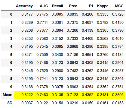
11.3 Random Forest Classifier

tuned_rf = tune_model(rf)

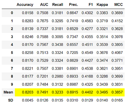
By default, tune_model optimizes Accuracy but this can be changed using optimize parameter. For example: tune_model(dt, optimize = 'AUC') will search for the hyperparameters of a Decision Tree Classifier that results in the highest AUC instead of Accuracy. For the purposes of this example, we have used the default metric Accuracy only for the sake of simplicity. Generally, when the dataset is imbalanced (such as the credit dataset we are working with) Accuracy is not a good metric for consideration. The methodology behind selecting the right metric to evaluate a classifier is beyond the scope of this tutorial but if you would like to learn more about it, you can click here to read an article on how to choose the right evaluation metric.

Metrics alone are not the only criteria you should consider when finalizing the best model for production. Other factors to consider include training time, the standard deviation of kfolds, etc. As you progress through the tutorial series we will discuss those factors in detail at the intermediate and expert levels. For now, let’s move forward considering the Tuned Random Forest Classifier tuned_rf, as our best model for the remainder of this tutorial.

12.0 Plot a Model

Before model finalization, the plot_model function can be used to analyze the performance across different aspects such as AUC, confusion_matrix, decision boundary, etc. This function takes a trained model object and returns a plot based on the test set.

There are 15 different plots available, please see the plot_model documentation for the list of available plots.

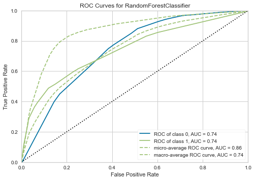
12.1 AUC Plot

plot_model(tuned_rf, plot = 'auc')

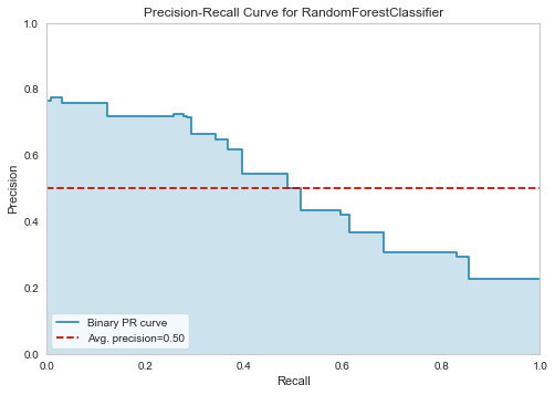
12.2 Precision-Recall Curve

plot_model(tuned_rf, plot = 'pr')

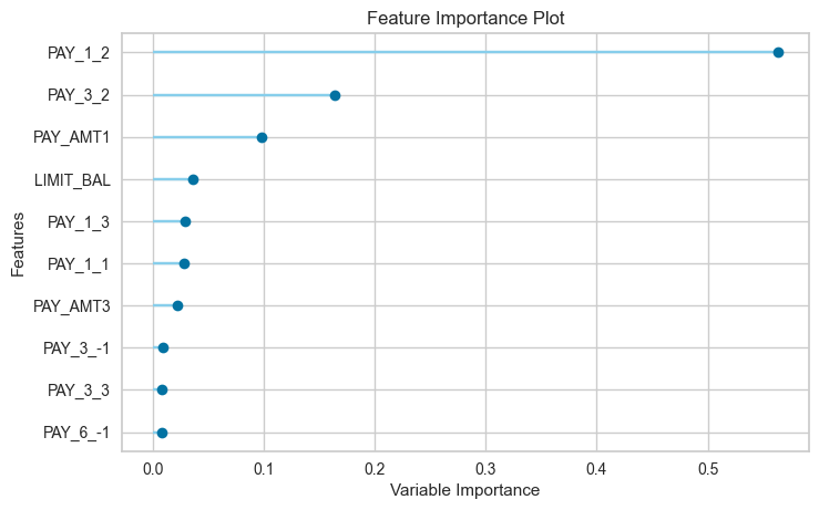
12.3 Feature Importance Plot

plot_model(tuned_rf, plot='feature')

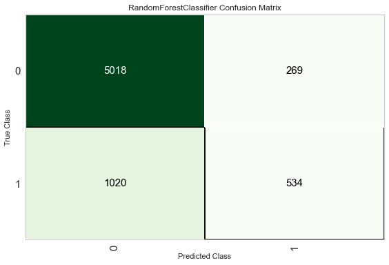
12.4 Confusion Matrix

plot_model(tuned_rf, plot = 'confusion_matrix')

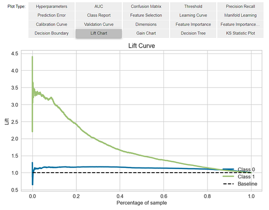
Another way to analyze the performance of models is to use the evaluate_model() function which displays a user interface for all of the available plots for a given model. It internally uses the plot_model() function.

evaluate_model(tuned_rf)

13.0 Predict on test / hold-out Sample

Before finalizing the model, it is advisable to perform one final check by predicting the test/hold-out set and reviewing the evaluation metrics. If you look at the information grid in Section 8 above, you will see that 30% (6,841 samples) of the data has been separated out as a test/hold-out sample. All of the evaluation metrics we have seen above are cross-validated results based on the training set (70%). Now, using our final trained model stored in the tuned_rf we will predict the test / hold-out sample and evaluate the metrics to see if they are materially different than the CV results.

predict_model(tuned_rf);

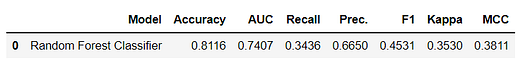
The accuracy on the test/hold-out set is 0.8116 compared to 0.8203 achieved on the tuned_rf CV results (in section 11.3 above). This is not a significant difference. If there is a large variation between the test/hold-out and CV results, then this would normally indicate over-fitting but could also be due to several other factors and would require further investigation. In this case, we will move forward with finalizing the model and predicting on unseen data (the 5% that we had separated in the beginning and never exposed to PyCaret).

(TIP: It’s always good to look at the standard deviation of CV results when using create_model)

14.0 Finalize Model for Deployment

Model finalization is the last step in the experiment. A normal machine learning workflow in PyCaret starts with setup, followed by comparing all models using the compare_models and shortlisting a few candidate models (based on the metric of interest) to perform several modeling techniques such as hyperparameter tuning, ensembling, stacking, etc. This workflow will eventually lead you to the best model for use in making predictions on new and unseen data. The finalize_model function fits the model onto the complete dataset including the test/hold-out sample (30% in this case). The purpose of this function is to train the final model on the complete dataset before it is deployed in production. (This is optional, you may or may not use finalize_model).

# finalize rf model
final_rf = finalize_model(tuned_rf)# print final model parameters
print(final_rf)>>> OUTPUTRandomForestClassifier(bootstrap=False, ccp_alpha=0.0, class_weight={},
                       criterion='entropy', max_depth=5, max_features=1.0,
                       max_leaf_nodes=None, max_samples=None,
                       min_impurity_decrease=0.0002, min_impurity_split=None,
                       min_samples_leaf=5, min_samples_split=10,
                       min_weight_fraction_leaf=0.0, n_estimators=150,
                       n_jobs=-1, oob_score=False, random_state=123, verbose=0,
                       warm_start=False)

Caution: One final word of caution. Once the model is finalized, the entire dataset including the test/hold-out set is used for training. As such, if the model is used for predictions on the hold-out set after finalize_model is used, the information grid printed will be misleading as you are trying to predict on the same data that was used for modeling. In order to demonstrate this point only, we will use final_rf under predict_model to compare the information grid with the one above in section 13.

predict_model(final_rf);

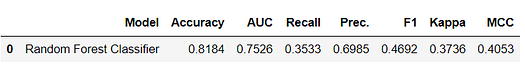
Notice how the AUC in final_rf has increased to 0.7526 from 0.7407, even though the model is the same. This is because the final_rf variable has been trained on the complete dataset including the test/hold-out set.

15.0 Predict on unseen data

The predict_model function is also used to predict on the unseen dataset. The only difference from section 13 above is that this time we will pass the data_unseen. It is the variable created at the beginning of this tutorial and contains 5% (1200 samples) of the original dataset which was never exposed to PyCaret. (see section 7 for explanation)

unseen_predictions = predict_model(final_rf, data=data_unseen)
unseen_predictions.head()

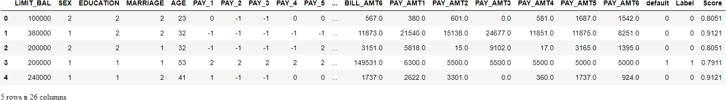
The Label and Score columns are added onto the data_unseen set. The label is the prediction and the score is the probability of the prediction. Notice that predicted results are concatenated to the original dataset while all the transformations are automatically performed in the background. You can also check the metrics on this since you have an actual target column default available. To do that we will use pycaret.utils module. See the example below:

# check metric on unseen data
from pycaret.utils import check_metric
check_metric(unseen_predictions['default'], unseen_predictions['Label'], metric = 'Accuracy')>>> OUTPUT
0.8167

16.0 Saving the model

We have now finished the experiment by finalizing the tuned_rf model which is now stored in final_rf variable. We have also used the model stored in final_rf to predict data_unseen. This brings us to the end of our experiment, but one question is still to be asked: What happens when you have more new data to predict? Do you have to go through the entire experiment again? The answer is no, PyCaret's inbuilt function save_model() allows you to save the model along with the entire transformation pipeline for later use.

# saving the final model
save_model(final_rf,'Final RF Model 11Nov2020')>>> Transformation Pipeline and Model Successfully Saved

17.0 Loading the saved model

To load a saved model at a future date in the same or an alternative environment, we would use PyCaret’s load_model() function and then easily apply the saved model on new unseen data for prediction.

# loading the saved model
saved_final_rf = load_model('Final RF Model 11Nov2020')>>> Transformation Pipeline and Model Successfully Loaded

Once the model is loaded in the environment, you can simply use it to predict on any new data using the same predict_model() function. Below we have applied the loaded model to predict the same data_unseen that we used in section 13 above.

# predict on new data
new_prediction = predict_model(saved_final_rf, data=data_unseen)
new_prediction.head()

Notice that the results of unseen_predictions and new_prediction are identical.

from pycaret.utils import check_metric
check_metric(new_prediction['default'], new_prediction['Label'], metric = 'Accuracy')>>> 0.8167

18.0 Wrap-up / Next Steps?

This tutorial has covered the entire machine learning pipeline from data ingestion, pre-processing, training the model, hyperparameter tuning, prediction, and saving the model for later use. We have completed all of these steps in less than 10 commands which are naturally constructed and very intuitive to remember such as create_model(), tune_model(), compare_models(). Re-creating the entire experiment without PyCaret would have taken well over 100 lines of code in most libraries.

We have only covered the basics of pycaret.classification. In the future tutorials we will go deeper into advanced pre-processing, ensembling, generalized stacking, and other techniques that allow you to fully customize your machine learning pipeline and are must know for any data scientist.

Thank you for reading ????

Important Links

⭐ Tutorials New to PyCaret? Check out our official notebooks!
???? Example Notebooks created by the community.
???? Blog Tutorials and articles by contributors.
???? Documentation The detailed API docs of PyCaret
???? Video Tutorials Our video tutorial from various events.
???? Discussions Have questions? Engage with community and contributors.
????️ Changelog Changes and version history.
???? Roadmap PyCaret’s software and community development plan.

Bio: Moez Ali writes about PyCaret and its use-cases in the real world, If you would like to be notified automatically, you can follow Moez on Medium, LinkedIn, and Twitter.

Original. Reposted with permission.

Related: