Geovisualization with Open Data
In this post I want to show how to use public available (open) data to create geo visualizations in python. Maps are a great way to communicate and compare information when working with geolocation data. There are many frameworks to plot maps, here I focus on matplotlib and geopandas (and give a glimpse of mplleaflet).
By Dr. Juan Camilo Orduz, Mathematician & Data Scientist
In this post I want to show how to use public available (open) data to create geo visualizations in python. Maps are a great way to communicate and compare information when working with geolocation data. There are many frameworks to plot maps, here I focus on matplotlib and geopandas (and give a glimpse of mplleaflet).
Reference: A very good introduction to matplotlib is the chapter on Visualization with Matplotlib from the Python Data Science Handbook by Jake VanderPlas.
Remark: When I finished writing this notebook, I discovered a similar analysis done in R here. Please check it out!
Prepare Notebook
import geopandas as gpd
import pandas as pd
import numpy as np
import matplotlib.pyplot as plt
plt.style.use('seaborn')

%matplotlib inline
Get Germany Data
The main data source for this post is www.suche-postleitzahl.org/downloads. Here we download three data sets:
plz-gebiete.shp: shapefile with germany postal codes polygons.zuordnung_plz_ort.csv: postal code to city and bundesland mapping.plz_einwohner.csv: population is assigned to each postal code area.
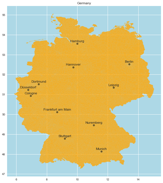
Germany Maps
We begin by generating a Germany map with the most important cities.
# Make sure you read postal codes as strings, otherwise
# the postal code 01110 will be parsed as the number 1110.
plz_shape_df = gpd.read_file('../Data/plz-gebiete.shp', dtype={'plz': str})

plz_shape_df.head()
| plz | note | geometry | |
|---|---|---|---|
| 0 | 52538 | 52538 Gangelt, Selfkant | POLYGON ((5.86632 51.05110, 5.86692 51.05124, … |
| 1 | 47559 | 47559 Kranenburg | POLYGON ((5.94504 51.82354, 5.94580 51.82409, … |
| 2 | 52525 | 52525 Waldfeucht, Heinsberg | POLYGON ((5.96811 51.05556, 5.96951 51.05660, … |
| 3 | 52074 | 52074 Aachen | POLYGON ((5.97486 50.79804, 5.97495 50.79809, … |
| 4 | 52531 | 52531 Ãbach-Palenberg | POLYGON ((6.01507 50.94788, 6.03854 50.93561, … |
The geometry column contains the polygons which define the postal code’s shape.
We can use geopandas mapping tools to generate the map with the plot method.
plt.rcParams['figure.figsize'] = [16, 11]

# Get lat and lng of Germany's main cities.
top_cities = {
    'Berlin': (13.404954, 52.520008),
    'Cologne': (6.953101, 50.935173),
    'Düsseldorf': (6.782048, 51.227144),
    'Frankfurt am Main': (8.682127, 50.110924),
    'Hamburg': (9.993682, 53.551086),
    'Leipzig': (12.387772, 51.343479),
    'Munich': (11.576124, 48.137154),
    'Dortmund': (7.468554, 51.513400),
    'Stuttgart': (9.181332, 48.777128),
    'Nuremberg': (11.077438, 49.449820),
    'Hannover': (9.73322, 52.37052)
}

fig, ax = plt.subplots()

plz_shape_df.plot(ax=ax, color='orange', alpha=0.8)

# Plot cities.
for c in top_cities.keys():
    # Plot city name.
    ax.text(
        x=top_cities[c][0],
        # Add small shift to avoid overlap with point.
        y=top_cities[c][1] + 0.08,
        s=c,
        fontsize=12,
        ha='center',
    )
    # Plot city location centroid.
    ax.plot(
        top_cities[c][0],
        top_cities[c][1],
        marker='o',
        c='black',
        alpha=0.5
    )

ax.set(
    title='Germany',
    aspect=1.3,
    facecolor='lightblue'
);
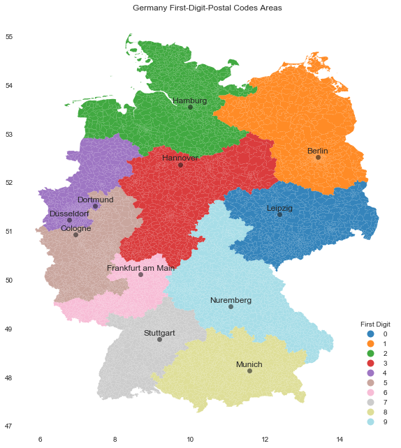
First-Digit-Postalcodes Areas
Next, let us plot different regions corresponding to the first digit of each postal code.
# Create feature.
plz_shape_df = plz_shape_df \
    .assign(first_dig_plz = lambda x: x['plz'].str.slice(start=0, stop=1))
fig, ax = plt.subplots()

plz_shape_df.plot(
    ax=ax,
    column='first_dig_plz',
    categorical=True,
    legend=True,
    legend_kwds={'title':'First Digit', 'loc':'lower right'},
    cmap='tab20',
    alpha=0.9
)

for c in top_cities.keys():

    ax.text(
        x=top_cities[c][0],
        y=top_cities[c][1] + 0.08,
        s=c,
        fontsize=12,
        ha='center',
    )

    ax.plot(
        top_cities[c][0],
        top_cities[c][1],
        marker='o',
        c='black',
        alpha=0.5
    )

ax.set(
    title='Germany First-Digit-Postal Codes Areas',
    aspect=1.3,
    facecolor='white'
);
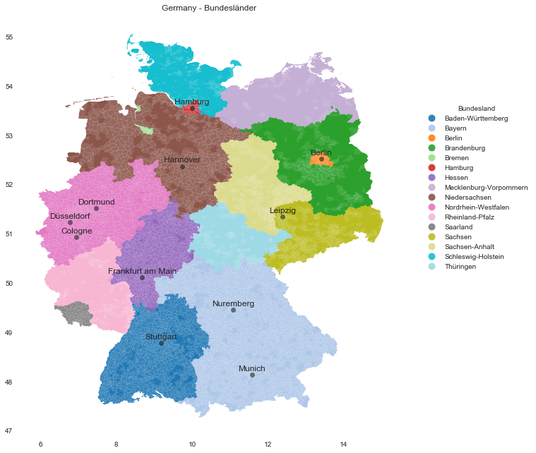
Bundesland Map
Let us now map each postal code to the corresponding region:
plz_region_df = pd.read_csv(
    '../Data/zuordnung_plz_ort.csv',
    sep=',',
    dtype={'plz': str}
)

plz_region_df.drop('osm_id', axis=1, inplace=True)

plz_region_df.head()
| ort | plz | bundesland | |
|---|---|---|---|
| 0 | Aach | 78267 | Baden-Württemberg |
| 1 | Aach | 54298 | Rheinland-Pfalz |
| 2 | Aachen | 52062 | Nordrhein-Westfalen |
| 3 | Aachen | 52064 | Nordrhein-Westfalen |
| 4 | Aachen | 52066 | Nordrhein-Westfalen |
# Merge data.
germany_df = pd.merge(
    left=plz_shape_df,
    right=plz_region_df,
    on='plz',
    how='inner'
)

germany_df.drop(['note'], axis=1, inplace=True)

germany_df.head()
| plz | geometry | first_dig_plz | ort | bundesland | |
|---|---|---|---|---|---|
| 0 | 52538 | POLYGON ((5.86632 51.05110, 5.86692 51.05124, … | 5 | Gangelt | Nordrhein-Westfalen |
| 1 | 52538 | POLYGON ((5.86632 51.05110, 5.86692 51.05124, … | 5 | Selfkant | Nordrhein-Westfalen |
| 2 | 47559 | POLYGON ((5.94504 51.82354, 5.94580 51.82409, … | 4 | Kranenburg | Nordrhein-Westfalen |
| 3 | 52525 | POLYGON ((5.96811 51.05556, 5.96951 51.05660, … | 5 | Heinsberg | Nordrhein-Westfalen |
| 4 | 52525 | POLYGON ((5.96811 51.05556, 5.96951 51.05660, … | 5 | Waldfeucht | Nordrhein-Westfalen |
Generate Bundesland map:
fig, ax = plt.subplots()

germany_df.plot(
    ax=ax,
    column='bundesland',
    categorical=True,
    legend=True,
    legend_kwds={'title':'Bundesland', 'bbox_to_anchor': (1.35, 0.8)},
    cmap='tab20',
    alpha=0.9
)

for c in top_cities.keys():

    ax.text(
        x=top_cities[c][0],
        y=top_cities[c][1] + 0.08,
        s=c,
        fontsize=12,
        ha='center',
    )

    ax.plot(
        top_cities[c][0],
        top_cities[c][1],
        marker='o',
        c='black',
        alpha=0.5
    )

ax.set(
    title='Germany - Bundesländer',
    aspect=1.3,
    facecolor='white'
);
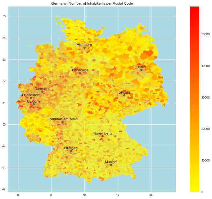
Number of Inhabitants
Now we include the number of inhabitants per postal code:
plz_einwohner_df = pd.read_csv(
    '../Data/plz_einwohner.csv',
    sep=',',
    dtype={'plz': str, 'einwohner': int}
)

plz_einwohner_df.head()
| plz | einwohner | |
|---|---|---|
| 0 | 01067 | 11957 |
| 1 | 01069 | 25491 |
| 2 | 01097 | 14811 |
| 3 | 01099 | 28021 |
| 4 | 01108 | 5876 |
# Merge data.
germany_df = pd.merge(
    left=germany_df,
    right=plz_einwohner_df,
    on='plz',
    how='left'
)

germany_df.head()
| plz | geometry | first_dig_plz | ort | bundesland | einwohner | |
|---|---|---|---|---|---|---|
| 0 | 52538 | POLYGON ((5.86632 51.05110, 5.86692 51.05124, … | 5 | Gangelt | Nordrhein-Westfalen | 21390 |
| 1 | 52538 | POLYGON ((5.86632 51.05110, 5.86692 51.05124, … | 5 | Selfkant | Nordrhein-Westfalen | 21390 |
| 2 | 47559 | POLYGON ((5.94504 51.82354, 5.94580 51.82409, … | 4 | Kranenburg | Nordrhein-Westfalen | 10220 |
| 3 | 52525 | POLYGON ((5.96811 51.05556, 5.96951 51.05660, … | 5 | Heinsberg | Nordrhein-Westfalen | 49737 |
| 4 | 52525 | POLYGON ((5.96811 51.05556, 5.96951 51.05660, … | 5 | Waldfeucht | Nordrhein-Westfalen | 49737 |
Generate map:
fig, ax = plt.subplots()

germany_df.plot(
    ax=ax,
    column='einwohner',
    categorical=False,
    legend=True,
    cmap='autumn_r',
    alpha=0.8
)

for c in top_cities.keys():

    ax.text(
        x=top_cities[c][0],
        y=top_cities[c][1] + 0.08,
        s=c,
        fontsize=12,
        ha='center',
    )

    ax.plot(
        top_cities[c][0],
        top_cities[c][1],
        marker='o',
        c='black',
        alpha=0.5
    )

ax.set(
    title='Germany: Number of Inhabitants per Postal Code',
    aspect=1.3,
    facecolor='lightblue'
);
City Maps
We can now filter for cities using the ort feature.
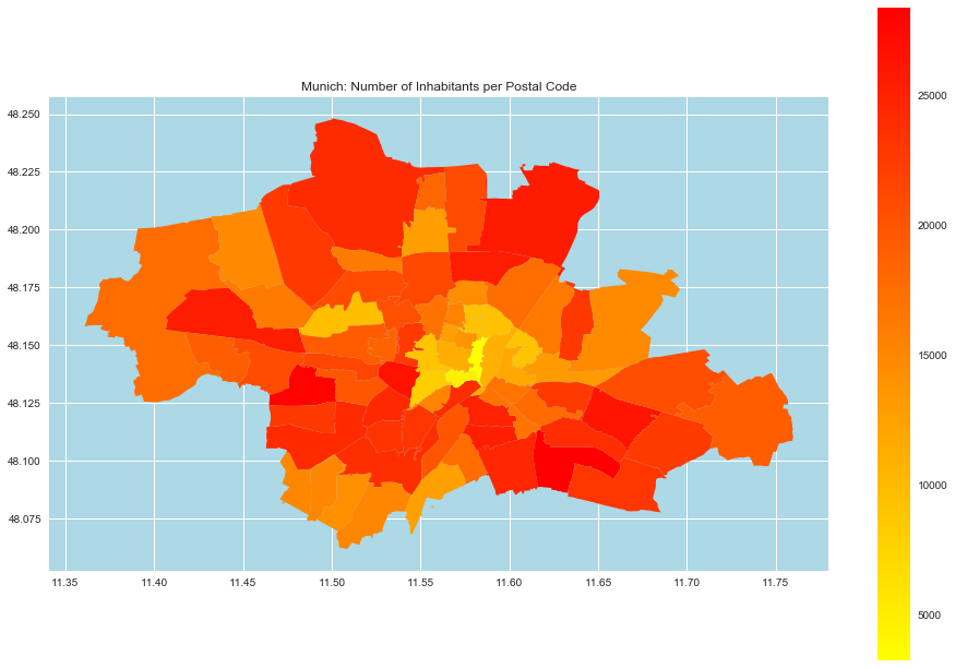
- Munich
munich_df = germany_df.query('ort == "München"')

fig, ax = plt.subplots()

munich_df.plot(
    ax=ax,
    column='einwohner',
    categorical=False,
    legend=True,
    cmap='autumn_r',
)

ax.set(
    title='Munich: Number of Inhabitants per Postal Code',
    aspect=1.3,
    facecolor='lightblue'
);
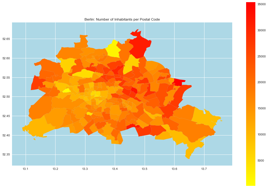
- Berlin
berlin_df = germany_df.query('ort == "Berlin"')

fig, ax = plt.subplots()

berlin_df.plot(
    ax=ax,
    column='einwohner',
    categorical=False,
    legend=True,
    cmap='autumn_r',
)

ax.set(
    title='Berlin: Number of Inhabitants per Postal Code',
    aspect=1.3,
    facecolor='lightblue'
);
Berlin
We can use the portal https://www.statistik-berlin-brandenburg.de to get the official postal code to area mapping in Berlin here. After some formating (not structured raw data):
berlin_plz_area_df = pd.read_excel(
    '../Data/ZuordnungderBezirkezuPostleitzahlen.xls',
    sheet_name='plz_bez_tidy',
    dtype={'plz': str}
)

berlin_plz_area_df.head()
| plz | area | |
|---|---|---|
| 0 | 10115 | Mitte |
| 1 | 10117 | Mitte |
| 2 | 10119 | Mitte |
| 3 | 10178 | Mitte |
| 4 | 10179 | Mitte |
Note however that this map is not one-to-one, i.e. a postal code can correspond to many areas:
berlin_plz_area_df \
    [berlin_plz_area_df['plz'].duplicated(keep=False)] \
    .sort_values('plz')
| plz | area | |
|---|---|---|
| 2 | 10119 | Mitte |
| 41 | 10119 | Pankow |
| 4 | 10179 | Mitte |
| 26 | 10179 | Friedrichshain-Kreuzberg |
| 42 | 10247 | Pankow |
| … | … | … |
| 133 | 14197 | Steglitz-Zehlendorf |
| 95 | 14197 | Charlottenburg-Wilmersdorf |
| 165 | 14197 | Tempelhof-Schöneberg |
| 134 | 14199 | Steglitz-Zehlendorf |
| 96 | 14199 | Charlottenburg-Wilmersdorf |
99 rows × 2 columns
Hence, we need to change the postal code grouping variable.
Berlin Neighbourhoods
Fortunately, the website http://insideairbnb.com/get-the-data.html, containing AirBnB data for many cities (which is definitely worth investigatinig!), has a convinient data set neighbourhoods.geojson which maps Berlin’s area to neighbourhoods:
berlin_neighbourhoods_df = gpd.read_file('../Data/neighbourhoods.geojson')

berlin_neighbourhoods_df = berlin_neighbourhoods_df \
    [~ berlin_neighbourhoods_df['neighbourhood_group'].isnull()]

berlin_neighbourhoods_df.head()
| neighbourhood | neighbourhood_group | geometry | |
|---|---|---|---|
| 0 | Blankenfelde/Niederschönhausen | Pankow | MULTIPOLYGON (((13.41191 52.61487, 13.41183 52… |
| 1 | Helmholtzplatz | Pankow | MULTIPOLYGON (((13.41405 52.54929, 13.41422 52… |
| 2 | Wiesbadener Straße | Charlottenburg-Wilm. | MULTIPOLYGON (((13.30748 52.46788, 13.30743 52… |
| 3 | Schmöckwitz/Karolinenhof/Rauchfangswerder | Treptow - Köpenick | MULTIPOLYGON (((13.70973 52.39630, 13.70926 52… |
| 4 | Müggelheim | Treptow - Köpenick | MULTIPOLYGON (((13.73762 52.40850, 13.73773 52… |
fig, ax = plt.subplots()

berlin_df.plot(
    ax=ax,
    alpha=0.2
)

berlin_neighbourhoods_df.plot(
    ax=ax,
    column='neighbourhood_group',
    categorical=True,
    legend=True,
    legend_kwds={'title': 'Neighbourhood', 'loc': 'upper right'},
    cmap='tab20',
    edgecolor='black'
)

ax.set(
    title='Berlin Neighbourhoods',
    aspect=1.3
);
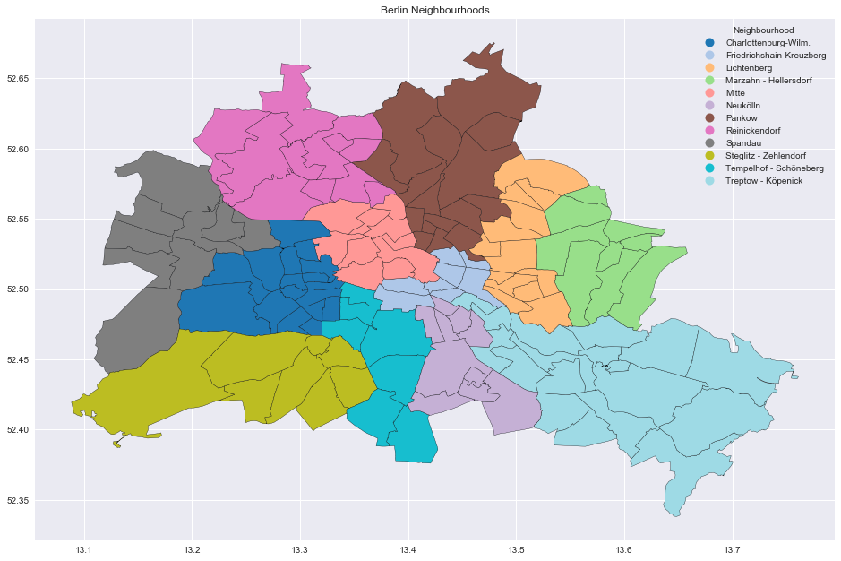
Neighbourhood ⊂⊂ Neighbourhood Group.
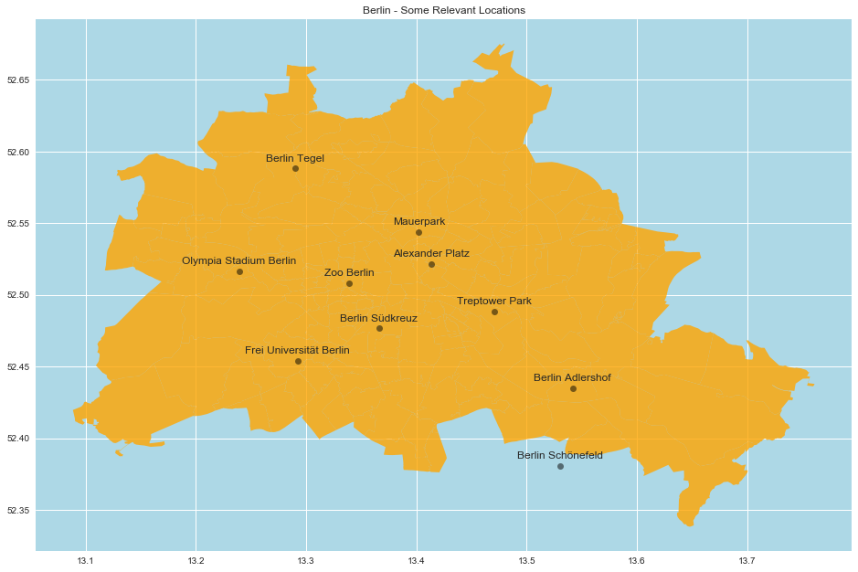
Selected Locations in Berlin
Sometimes it is useful to include well-known locations on the maps so that the user can identify them and understand the distances and scales. One way to do it is to manualy input the latitude and longitude of each point (as above). This of course can be time consuming and prone to errors. As expected, there is a library which can fetch this type of data automatically, namely geopy.
Here is a simple example:
from geopy import Nominatim

locator = Nominatim(user_agent='myGeocoder')

location = locator.geocode('Humboldt Universität zu Berlin')

print(location)
Humboldt-Universität zu Berlin, Dorotheenstraße, Spandauer Vorstadt, Mitte, Berlin, 10117, Deutschland
Let us write a function to get the latitude and longitude coordinates:
def lat_lng_from_string_loc(x):

    locator = Nominatim(user_agent='myGeocoder')

    location = locator.geocode(x)

    if location is None:
        None
    else:
        return location.longitude, location.latitude
# Define some well-known Berlin locations.
berlin_locations = [
    'Alexander Platz',
    'Zoo Berlin',
    'Berlin Tegel',
    'Berlin Schönefeld',
    'Berlin Adlershof',
    'Olympia Stadium Berlin',
    'Berlin Südkreuz',
    'Frei Universität Berlin',
    'Mauerpark',
    'Treptower Park',
]

# Get geodata.
berlin_locations_geo = {
    x: lat_lng_from_string_loc(x)
    for x in berlin_locations
}

# Remove None.
berlin_locations_geo = {
    k: v
    for k, v in berlin_locations_geo.items()
    if v is not None
}
Let us see the resulting map:
berlin_df = germany_df.query('ort == "Berlin"')

fig, ax = plt.subplots()

berlin_df.plot(
    ax=ax,
    color='orange',
    alpha=0.8
)

for c in berlin_locations_geo.keys():

    ax.text(
        x=berlin_locations_geo[c][0],
        y=berlin_locations_geo[c][1] + 0.005,
        s=c,
        fontsize=12,
        ha='center',
    )

    ax.plot(
        berlin_locations_geo[c][0],
        berlin_locations_geo[c][1],
        marker='o',
        c='black',
        alpha=0.5
    )

ax.set(
    title='Berlin - Some Relevant Locations',
    aspect=1.3,
    facecolor='lightblue'
);
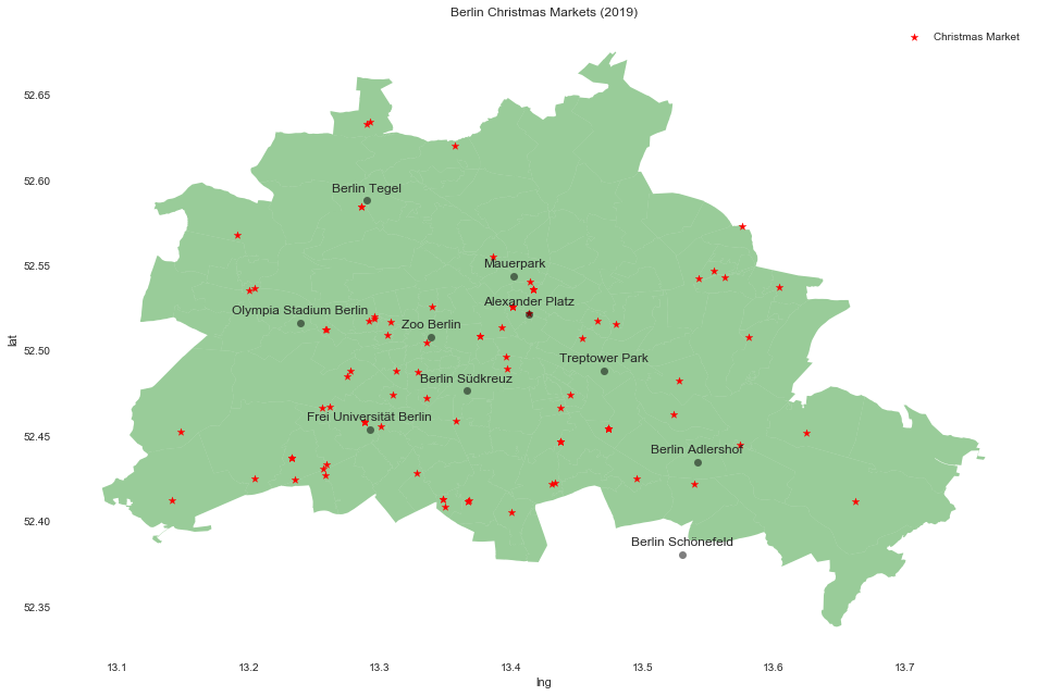
Christmas Markets
Let us enrich the maps by including other type of information. There is a great resource for publicly available data for Berlin: Berlin Open Data. Among many interesting datasets, I found one on the Christmas markets around the city (which are really fun to visit!) here. You can accces the data via a public API. Let us use the requests module to do this:
import requests

# GET request.
response = requests.get(
    'https://www.berlin.de/sen/web/service/maerkte-feste/weihnachtsmaerkte/index.php/index/all.json?q='
)

response_json = response.json()
Convert to pandas dataframe.
berlin_maerkte_raw_df = pd.DataFrame(response_json['index'])
We do not have a postal code feature, but we can create one by extracting it from the plz_ort column.
berlin_maerkte_df = berlin_maerkte_raw_df[['name', 'bezirk', 'plz_ort', 'lat', 'lng']]

berlin_maerkte_df = berlin_maerkte_df \
    .query('lat != ""') \
    .assign(plz = lambda x: x['plz_ort'].str.split(' ').apply(lambda x: x[0]).astype(str)) \
    .drop('plz_ort', axis=1)

# Convert to float.
berlin_maerkte_df['lat'] = berlin_maerkte_df['lat'].str.replace(',', '.').astype(float)
berlin_maerkte_df['lng'] = berlin_maerkte_df['lng'].str.replace(',', '.').astype(float)

berlin_maerkte_df.head()
| name | bezirk | lat | lng | plz | |
|---|---|---|---|---|---|
| 0 | Weihnachtsmarkt vor dem Schloss Charlottenburg | Charlottenburg-Wilmersdorf | 52.519951 | 13.295946 | 14059 |
| 1 |
|
Charlottenburg-Wilmersdorf | 52.504886 | 13.335511 | 10789 |
| 2 | Weihnachtsmarkt in der Fußgängerzone Wilmersdo… | Charlottenburg-Wilmersdorf | 52.509313 | 13.305994 | 10627 |
| 3 | Weihnachten in Westend | Charlottenburg-Wilmersdorf | 52.512538 | 13.259213 | 14052 |
| 4 | Weihnachtsmarkt Berlin-Grunewald des Johannisc… | Charlottenburg-Wilmersdorf | 52.488350 | 13.277250 | 14193 |
Let us plot the Christmas markets locations:
fig, ax = plt.subplots()

berlin_df.plot(ax=ax, color= 'green', alpha=0.4)

for c in berlin_locations_geo.keys():

    ax.text(
        x=berlin_locations_geo[c][0],
        y=berlin_locations_geo[c][1] + 0.005,
        s=c,
        fontsize=12,
        ha='center',
    )

    ax.plot(
        berlin_locations_geo[c][0],
        berlin_locations_geo[c][1],
        marker='o',
        c='black',
        alpha=0.5
    )

berlin_maerkte_df.plot(
    kind='scatter',
    x='lng',
    y='lat',
    c='r',
    marker='*',
    s=50,
    label='Christmas Market',
    ax=ax
)

ax.set(
    title='Berlin Christmas Markets (2019)',
    aspect=1.3,
    facecolor='white'
);
Interactive Maps
We can use the mplleaflet library which converts a matplotlib plot into a webpage containing a pannable, zoomable Leaflet map.
- Berlin Neighbourhoods
import mplleaflet

fig, ax = plt.subplots()

berlin_df.plot(
    ax=ax,
    alpha=0.2
)

berlin_neighbourhoods_df.plot(
    ax=ax,
    column='neighbourhood_group',
    categorical=True,
    cmap='tab20',
)

mplleaflet.display(fig=fig)
- Christmas Markets
fig, ax = plt.subplots()

berlin_df.plot(ax=ax, color= 'green', alpha=0.4)

berlin_maerkte_df.plot(
    kind='scatter',
    x='lng',
    y='lat',
    c='r',
    marker='*',
    s=30,
    ax=ax
)

mplleaflet.display(fig=fig)
Bio: Dr. Juan Camilo Orduz (@juanitorduz) in a Berlin based mathematician & data scientist.
Original. Reposted with permission.
Related:
- 6 Books About Open Data Every Data Scientist Should Read
- Eight iconic examples of data visualisation
- Metadata Enrichment is Essential to Realize the Value of Open Datasets