Brain Tumor Detection using Mask R-CNN
Mask R-CNN has been the new state of the art in terms of instance segmentation. Here I want to share some simple understanding of it to give you a first look and then we can move ahead and build our model.
“Radiology is the medical discipline that uses medical imaging to diagnose and treat diseases within the bodies of both humans and animals.” — Wikipedia
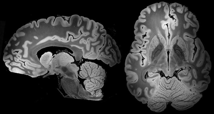
In the health care sector, medical image analysis plays an active role, especially in Non-invasive treatment and clinical study. Medical imaging techniques and analysis tools help medical practitioners and radiologists to correctly diagnose the disease. Medical Image Processing has appeared as one of the most critical tools to recognize and diagnose various abnormalities. Imaging empowers doctors to visualize and examine the MRI images for finding the deformities/abnormalities in internal structures. An important factor in the diagnosis includes the medical image data obtained from various biomedical tools which use different imaging techniques like X-rays, CT scans, MRI, mammogram, etc.
Artificial intelligence (AI) algorithms, particularly Deep learning, have shown remarkable progress in image-recognition jobs. Practices ranging from convolutional neural networks(CNN) to variational autoencoders have found innumerable applications in the medical image analysis field, driving it forward at a rapid pace. In radiology, trained physicians visually evaluated medical images for the detection, characterization, and monitoring of diseases. AI algos outshines at automatically recognizing complex patterns in imaging data and producing quantitative, rather than qualitative, evaluations of radiographic features.
Diagnosing a brain tumor begins with Magnetic Resonance Imaging (MRI). Once MRI shows that there is a tumor in the brain, the most regular way to infer the type of brain tumor is to glance at the results from a sample of tissue after a biopsy/surgery.
An MRI uses magnetic fields, to produce accurate images of the body organs. It can be used to measure the tumor’s size. A special dye called a contrast medium is given before the scan to create an accurate snd clearer picture. This dye can be injected into a patient’s vein or given as a pill or liquid.
MRIs create more accurate snd clearer pictures than CT scans and are the favored way to diagnose a brain tumor. The MRI may be of the brain, spinal cord, or both, depending on the type of tumor presumed and the plausibility that it will spread in the CNS. There are different types of MRIs and the results of a neuro-test, done by the neurologist, help determine which type of MRI to use.
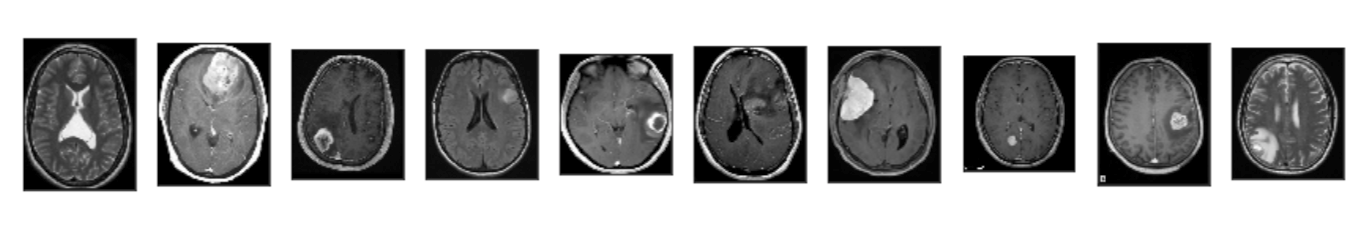
In this article, we are going to build a Mask R-CNN model capable of detecting tumours from MRI scans of the brain images.
Mask R-CNN has been the new state of the art in terms of instance segmentation. There are rigorous papers, easy to understand tutorials with good quality open-source codes around for your reference. Here I want to share some simple understanding of it to give you a first look and then we can move ahead and build our model.
Understanding Mask R-CNN
Mask R-CNN is an extension of Faster R-CNN. Faster R-CNN is widely used for object detection tasks. For a given image, it returns the class label and bounding box coordinates for each object in the image. So, let’s say you pass the following image:

The Fast R-CNN model will return something like this:

For a given image, Mask R-CNN, in addition to the class label and bounding box coordinates for each object, will also return the object mask.
The model is divided into two parts:
- Region proposal network (RPN) to proposes candidate object bounding boxes.
- Binary mask classifier to generate a mask for every class

Mask R-CNN has a branch for classification and bounding box regression. It uses:
- ResNet101 architecture to extract features from an image.
- Region Proposal Network(RPN) to generate Region of Interests(RoI)
Let’s first quickly understand how Faster R-CNN works. This will help us grasp the intuition behind Mask R-CNN as well.
- Faster R-CNN first uses a ConvNet to extract feature maps from the images
- These feature maps are then passed through a Region Proposal Network (RPN) which returns the candidate bounding boxes
- We then apply an RoI pooling layer on these candidate bounding boxes to bring all the candidates to the same size
- And finally, the proposals are passed to a fully connected layer to classify and output the bounding boxes for objects
Building a Brain Tumour Detector using Mark R-CNN
A brain tumor occurs when abnormal cells form within the brain. There are two main types of tumors: cancerous (malignant) tumors and benign tumors. Malignant tumors can be divided into primary tumors, which start within the brain, and secondary tumors, which have spread from elsewhere, known as brain metastasis tumors.

To start with first you need to clone Mask_RCNN and brain tumor image as shown below:
Step 1: Clone the Mask R-CNN repository and Brain MRI scan as input data.
from IPython.display import clear_output!git clone https://github.com/matterport/Mask_RCNN.git # load Mask R-CNN code implementation!git clone https://github.com/ruslan-kl/brain-tumor.git # load new data set and annotations!pip install pycocotools!rm -rf brain-tumor/.git/
!rm -rf Mask_RCNN/.git/clear_output()
Step-2: Create the directory structure of your input image data.
MODEL_DIR = os.path.join(ROOT_DIR, 'logs') # directory to save logs and trained model
# ANNOTATIONS_DIR = 'brain-tumor/data/new/annotations/' # directory with annotations for train/val sets
DATASET_DIR = 'brain-tumor/data_cleaned/' # directory with image data
DEFAULT_LOGS_DIR = 'logs'# Local path to trained weights file
COCO_MODEL_PATH = os.path.join(ROOT_DIR, "mask_rcnn_coco.h5")
# Download COCO trained weights from Releases if needed
if not os.path.exists(COCO_MODEL_PATH):
    utils.download_trained_weights(COCO_MODEL_PATH)
Let us have a look at the dataset that we have just loaded.

Step-3: Configuration for training on the brain tumor dataset.
Here we need to set up configuration include properties like setting the number of GPUs to use along with the number of images per GPU, Number of classes (we would normally add +1 for the background), Number of training steps per epoch, Learning rate, Skip detections with < 85% confidence,
class TumorConfig(Config):
    # Give the configuration a recognizable name
    NAME = 'tumor_detector'
    GPU_COUNT = 1
    IMAGES_PER_GPU = 1
    NUM_CLASSES = 1 + 1  # background + tumor
    DETECTION_MIN_CONFIDENCE = 0.85
    STEPS_PER_EPOCH = 100
    LEARNING_RATE = 0.001

config = TumorConfig()
config.display()
Step: 4: Build the custom brain MRI data set.
Dataset class provides a consistent way to work with any dataset. We will create our new datasets for brain images to train without having to change the code of the model.
Dataset class also supports loading multiple data sets at the same time. This is very helpful when you want to detect different objects and they are all not available in one data set.
In the load_dataset method, we iterate through all the files in the image and annotations folders to add the class, images, and annotations to create the dataset using add_class and add_image methods.
extract_boxes method extracts each of the bounding boxes from the annotation file. Annotation files are XML files using Pascal VOC format. It returns the box, it’s height and width
load_mask method generates the masks for every object in the image. It returns one mask per instance and class ids, a 1D array of class id for the instance masks
image_reference method returns the path of the image.
class BrainScanDataset(utils.Dataset):def load_brain_scan(self, dataset_dir, subset):
        """Load a subset of the FarmCow dataset.
        dataset_dir: Root directory of the dataset.
        subset: Subset to load: train or val
        """
        # Add classes. We have only one class to add.
        self.add_class("tumor", 1, "tumor")# Train or validation dataset?
        assert subset in ["train", "val", 'test']
        dataset_dir = os.path.join(dataset_dir, subset)annotations = json.load(open(os.path.join(DATASET_DIR, subset, 'annotations_'+subset+'.json')))
        annotations = list(annotations.values())  # don't need the dict keys# The VIA tool saves images in the JSON even if they don't have any
        # annotations. Skip unannotated images.
        annotations = [a for a in annotations if a['regions']]# Add images
        for a in annotations:
            # Get the x, y coordinaets of points of the polygons that make up
            # the outline of each object instance. These are stores in the
            # shape_attributes (see json format above)
            # The if condition is needed to support VIA versions 1.x and 2.x.
            if type(a['regions']) is dict:
                polygons = [r['shape_attributes'] for r in a['regions'].values()]
            else:
                polygons = [r['shape_attributes'] for r in a['regions']]# load_mask() needs the image size to convert polygons to masks.
            # Unfortunately, VIA doesn't include it in JSON, so we must read
            # the image. This is only managable since the dataset is tiny.
            image_path = os.path.join(dataset_dir, a['filename'])
            image = skimage.io.imread(image_path)
            height, width = image.shape[:2]self.add_image(
                "tumor",
                image_id=a['filename'],  # use file name as a unique image id
                path=image_path,
                width=width,
                height=height,
                polygons=polygons
            )def load_mask(self, image_id):
        """Generate instance masks for an image.
       Returns:
        masks: A bool array of shape [height, width, instance count] with
            one mask per instance.
        class_ids: a 1D array of class IDs of the instance masks.
        """
        # If not a farm_cow dataset image, delegate to parent class.
        image_info = self.image_info[image_id]
        if image_info["source"] != "tumor":
            return super(self.__class__, self).load_mask(image_id)# Convert polygons to a bitmap mask of shape
        # [height, width, instance_count]
        info = self.image_info[image_id]
        mask = np.zeros([info["height"], info["width"], len(info["polygons"])],
                        dtype=np.uint8)
        for i, p in enumerate(info["polygons"]):
            # Get indexes of pixels inside the polygon and set them to 1
            rr, cc = skimage.draw.polygon(p['all_points_y'], p['all_points_x'])
            mask[rr, cc, i] = 1# Return mask, and array of class IDs of each instance. Since we have
        # one class ID only, we return an array of 1s
        return mask.astype(np.bool), np.ones([mask.shape[-1]], dtype=np.int32)def image_reference(self, image_id):
        """Return the path of the image."""
        info = self.image_info[image_id]
        if info["source"] == "tumor":
            return info["path"]
        else:
            super(self.__class__, self).image_reference(image_id)
Step-5: Initialize the Mask R-CNN model for training using the Config instance that we created and load the pre-trained weights for the Mask R-CNN from the COCO data set excluding the last few layers.
Since we’re using a very small dataset, and starting from COCO trained weights, we don’t need to train too long. Also, no need to train all layers, just the heads should do it.
We exclude the last few layers from training for ResNet101.
model = modellib.MaskRCNN(
    mode='training',
    config=config,
    model_dir=DEFAULT_LOGS_DIR
)model.load_weights(
    COCO_MODEL_PATH,
    by_name=True,
    exclude=["mrcnn_class_logits", "mrcnn_bbox_fc", "mrcnn_bbox", "mrcnn_mask"]
)
Step: 6: Load the dataset and train your model for 15 epochs with the Learning rate as 0.001
# Training dataset.
dataset_train = BrainScanDataset()
dataset_train.load_brain_scan(DATASET_DIR, 'train')
dataset_train.prepare()# Validation dataset
dataset_val = BrainScanDataset()
dataset_val.load_brain_scan(DATASET_DIR, 'val')
dataset_val.prepare()dataset_test = BrainScanDataset()
dataset_test.load_brain_scan(DATASET_DIR, 'test')
dataset_test.prepare()print("Training network heads")
model.train(
    dataset_train, dataset_val,
    learning_rate=config.LEARNING_RATE,
    epochs=15,
    layers='heads'
)
Step 7: Recreate the model in inference mode
# Recreate the model in inference mode
model = modellib.MaskRCNN(
    mode="inference",
    config=config,
    model_dir=DEFAULT_LOGS_DIR
)model_path = model.find_last()# Load trained weights
print("Loading weights from ", model_path)
model.load_weights(model_path, by_name=True)
Step 8: Now build functions to display the results.
def predict_and_plot_differences(dataset, img_id):
    original_image, image_meta, gt_class_id, gt_box, gt_mask =\
        modellib.load_image_gt(dataset, config,
                               img_id, use_mini_mask=False)    results = model.detect([original_image], verbose=0)
    r = results[0]    visualize.display_differences(
        original_image,
        gt_box, gt_class_id, gt_mask,
        r['rois'], r['class_ids'], r['scores'], r['masks'],
        class_names = ['tumor'], title="", ax=get_ax(),
        show_mask=True, show_box=True)
    def display_image(dataset, ind):
    plt.figure(figsize=(5,5))
    plt.imshow(dataset.load_image(ind))
    plt.xticks([])
    plt.yticks([])
    plt.title('Original Image')
    plt.show()
Test your model prediction on the validation set:
#Validation set
ind = 9
display_image(dataset_val, ind)
predict_and_plot_differences(dataset_val, ind)

ind = 6
display_image(dataset_val, ind)
predict_and_plot_differences(dataset_val, ind)

Now test the model in the test set.
#Test Set
ind = 1
display_image(dataset_test, ind)
predict_and_plot_differences(dataset_test, ind)

ind = 0
display_image(dataset_test, ind)
predict_and_plot_differences(dataset_test, ind)

As you can see we are getting pretty good accuracy.
You can get the whole code in this GitHub repo.
Conclusion
AI will surely impact radiology, and more quickly than other medical fields. It will change radiology practice faster than ever before. Radiologists can play a principal role in this upcoming change.
An agitation among radiologists to embrace AI may be compared with the hesitation among pilots to embrace autopilot technology in the early days of automated aircraft aviation. However, radiologists are used to handling technological barriers because, following the beginnings of its past, radiology has been the playground of technological evolution.
An updated radiologist should be conscious of the basic principles of AI systems, the quality of datasets to train them, and their restrictions. Radiologists do not need to know the most profound details of these systems, but they must learn the technical lexicon used by data scientists to efficiently interact with them. The time to work for and with AI in radiology is now.
Well, this concludes this article. I hope you guys have enjoyed reading it, feel free to share your comments/thoughts/feedback in the comment section.
Thanks for reading this article!!!
Bio: Nagesh Singh Chauhan is a Big data developer at CirrusLabs. He has over 4 years of working experience in various sectors like Telecom, Analytics, Sales, Data Science having specialisation in various Big data components.
Original. Reposted with permission.
Related:
- Convolutional Neural Network for Breast Cancer Classification
- Fourier Transformation for a Data Scientist
- Build an Artificial Neural Network From Scratch: Part 2