Recreating Fingerprints using Convolutional Autoencoders
The article gets you started working with fingerprints using Deep Learning.

Biometrics is the technical term for body measurements and calculations. It refers to metrics related to human characteristics. Biometrics authentication (or realistic authentication) is used in computer science as a form of identification and access control. It is also used to identify individuals in groups that are under surveillance.
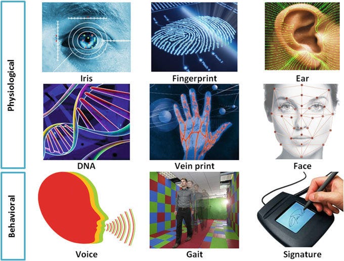
Biometric authentication systems are classified into two types such as Physiological Biometrics and Behavioral Biometrics. Physiological biometrics mainly include face recognition, fingerprint, hand geometry, iris recognition, and DNA. Whereas behavioral biometrics include keystroke, signature and voice recognition.
Fingerprints are the most reliable human characteristics that can be used for personal identification and has been widely used in biometric authentication systems due to its uniqueness and consistency. Fingerprint recognition systems play a crucial role in many situations where a person needs to be verified or identified with high confidence.
Despite the tremendous progress made in Automatic Fingerprint Identification Systems (AFIS), highly efficient and accurate fingerprint matching remains a critical challenge.
Fingerprints: As Unique as You
Imagine you misplaced your smartphone and start panicking because there’s a lot of personal information on that phone. You’re worried because you don’t want whoever picks it up to be able to access it. But then you remember that you secured it so that no one could use it, should this scenario ever arise. The only person your phone will unlock for is you, and it knows it’s you because you use your fingerprint.
Fingerprints and also toe prints can be used to identify a single individual because they are unique to each person and they do not change over time. Amazingly, even identical twins have fingerprints that are different from each other, and none of your fingers have the same print as the others. Fingerprints consist of ridges, which are the raised lines, and furrows, which are the valleys between those lines. And it’s the pattern of those ridges and furrows that are different for everyone.
The patterns of the ridges are what is imprinted on a surface when your finger touches it. If you get fingerprinted the ridges are printed on the paper and can be used to match fingerprints you might leave elsewhere.
Human fingerprints are detailed, almost unique, difficult to modify, and durable over the life of an individual, making them suitable as long-term markers of human identity.
Characteristics of Fingerprints
The first encounter with fingerprints makes them look complicated. They may leave you wondering how forensic and law enforcement people make use of them. Fingerprints may look complicated, but the fact is that they have general ridge patterns and each person’s fingerprint is unique making it possible to systematically classify them.
Fingerprints have three basic ridge patterns: “Arch”, “Loop” and “Whorl/Core”.
Arches
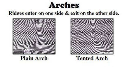
In this pattern type, ridges enter on one side and exit on the other side. 5% of the total world’s population is believed to have arches in their fingerprints.
Loops
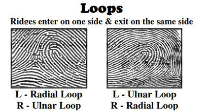
This pattern type has ridges entering on one side and exiting on the same side. 60–65% of the world’s population is believed to have loops in their fingerprints.
Whorls/Core
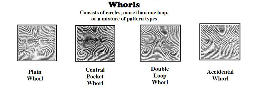
Consists of circles, more than one loop, or a mixture of pattern type. 30–35% of the world’s population is believed to have whorls in their fingerprints.
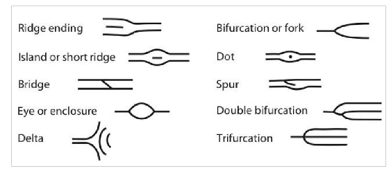
The uniqueness of a fingerprint is exclusively determined by the local ridge characteristics and their relationships. The ridges and valleys in a fingerprint alternate, flowing in a local constant direction. The two most prominent local ridge characteristics are: 1) ridge ending and, 2) ridge bifurcation. A ridge ending is defined as the point where a ridge ends abruptly. A ridge bifurcation is defined as the point where a ridge forks or diverges into branch ridges. Collectively, these features are called minutiae.
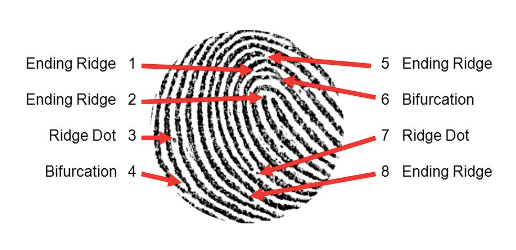
The set of minutiae points is considered to be the most distinctive feature for fingerprint representation and is widely used in fingerprint matching. It was believed that the minutiae set do not contain sufficient information to reconstruct the original fingerprint image from which minutiae were extracted. However, recent studies have shown that it is indeed possible to reconstruct fingerprint images from their minutiae representations.
Building a Convolutional Autoencoder
After having an overview of the fingerprint, its features, it is time to utilize our newly developed skill to build a Neural network that is capable of recreating or reconstructing fingerprint images.
So, first of all, we’ll explore the dataset including what kind of images it has, how to read the images, how to create an array of the images, exploring the fingerprint images and finally preprocessing them to be able to feed them in the model.
I have used convolutional autoencoder for training the model. Next, we will visualize the training and validation loss plot and finally predict the test set.
Here I’m assuming you guys are comfortable with Convolutional Neural Networks and AutoEncoders. Anyway, I’ll try to explain them as a one-liner.
A Convolutional neural network (CNN) is a neural network that has one or more convolutional layers and is used mainly for image processing, classification, and segmentation.
OK. Whats an AutoEncoder?
Autoencoders are a family of Neural Networks for which the input is the same as the output. They work by compressing the input into a latent-space representation and then reconstructing the output from this representation. Check this out for more.
Now whats a Convolutional Autoencoders?
The convolution operator allows filtering an input signal in order to extract some part of its content. Autoencoders in their traditional formulation do not take into account the fact that a signal can be seen as a sum of other signals. Convolutional Autoencoders, instead, use the convolution operator to exploit this observation. They learn to encode the input in a set of simple signals and then try to reconstruct the input from them. For more check this out.

The result is a 2x2x1 activation map. Source
The dataset that I’m using is the FVC2002 fingerprint dataset. It consists of 4 different sensor fingerprints namely Low-cost Optical Sensor, Low-cost Capacitive Sensor, Optical Sensor and Synthetic Generator, each sensor having varying image sizes. The dataset has 320 images, 80 images per sensor.
Load the required libraries:
import cv2
import matplotlib.pyplot as plt
%matplotlib inline
from skimage.filters import threshold_otsu
import numpy as np
from glob import glob
import scipy.misc
from matplotlib.patches import Circle,Ellipse
from matplotlib.patches import Rectangle
import os
from PIL import Imageimport keras
from matplotlib import pyplot as plt
import numpy as np
import gzip
%matplotlib inline
from keras.layers import Input,Conv2D,MaxPooling2D,UpSampling2D
from keras.models import Model
from keras.optimizers import RMSprop
from keras.layers.normalization import BatchNormalization
Load the dataset:
data = glob('./drive/My Drive/fingerprint/DB*/*')images = []
def readImages(data):
    for i in range(len(data)):
        img = scipy.misc.imread(data[i])
        img = scipy.misc.imresize(img,(224,224))
        images.append(img)
    return imagesimages = readImages(data)
Now convert these images into float32 array.
images_arr = np.asarray(images)
images_arr = images_arr.astype('float32')
images_arr.shape
Once you have the data loaded properly, you are all set to analyze it in order to get some intuition about the dataset.
Data Exploration:
print("Dataset (images) shape: {shape}".format(shape=images_arr.shape))##Dataset (images) shape: (320, 224, 224)From the above output, you can see that the data has a shape of 320 x 224 x 224 since there are 320 samples each of the 224 x 224-dimensional matrix.
Take a look at a first 5 images in our dataset:
# Display the first 5 images in training data
for i in range(5):
    plt.figure(figsize=[5, 5])
    curr_img = np.reshape(images_arr[i], (224,224))
    plt.imshow(curr_img, cmap='gray')
    plt.show()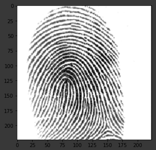
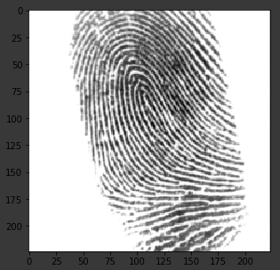
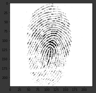
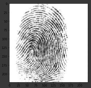
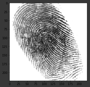
As we can see that the fingerprints are not very clear, it will be interesting to see if the convolutional autoencoder is able to learn the features and is able to reconstruct these images properly.
The images of the dataset are grayscale images with pixel values ranging from 0 to 255 having a dimension of 224 x 224, so before we feed the data into the model, it is very important to preprocess it. We’ll first convert each 224 x 224 image of the dataset into a matrix of size 224 x 224 x 1. 1 for Grayscale image, which we can then feed into the Neural Network:
images_arr = images_arr.reshape(-1, 224,224, 1)
images_arr.shape##(320, 224, 224, 1)
Next, we want to make sure to check the data type of the NumPy array; it should be in float32 format, if not you will need to convert it into this format, you also have to rescale the pixel values in range 0–1.
images_arr.dtypeIf we verify we should get dtype('float32')
Next, rescale the data with the maximum pixel value of the images in the data:
np.max(images_arr)
images_arr = images_arr / np.max(images_arr)
Let’s verify the maximum and minimum value of data which should be 0.0 and 1.0 after rescaling it!
np.max(images_arr), np.min(images_arr)If we verify we should get (1.0, 0.0)
In order for your model to generalize well, you split the data into two parts: training and a validation set. You will train your model on 80% of the data and validate it on 20% of the remaining training data.
This will also help you in reducing the chances of overfitting, as you will be validating your model on data it would not have seen in the training phase.
from sklearn.model_selection import train_test_split
train_X,valid_X,train_ground,valid_ground = train_test_split(images_arr,images_arr,test_size=0.2,random_state=13)
We don’t need training and testing labels that’s why we will pass the training images twice. Our training images will both act as the input as well as the ground truth similar to the labels you have in the classification task.
Now we are all set to define the network and feed the data into the network.
The Convolutional Autoencoder
The images are of size 224 x 224 x 1 or a 50,176-dimensional vector. We convert the image matrix to an array, rescale it between 0 and 1, reshape it so that it’s of size 224 x 224 x 1, and feed this as an input to the network.
Also, we will use a batch size of 128 using a higher batch size of 256 or 512 is also preferable it all depends on the system you train your model. It contributes heavily in determining the learning parameters and affects the prediction accuracy. We will train your network for 300 epochs.
batch_size = 128
epochs = 300
x, y = 224, 224
input_img = Input(shape = (x, y, 1))
As you might already know well before, the autoencoder is divided into two parts: there are encoder and a decoder.
Encoder
- The first layer will have 32 filters of size 3 x 3, followed by a downsampling (max-pooling) layer,
- The second layer will have 64 filters of size 3 x 3, followed by another downsampling layer,
- The final layer of encoder will have 128 filters of size 3 x 3.
Decoder
- The first layer will have 128 filters of size 3 x 3 followed by an upsampling layer,
- The second layer will have 64 filters of size 3 x 3 followed by another upsampling layer,
- The final layer of encoder will have one filter of size 3 x 3.
The max-pooling layer will downsample the input by two times each time you use it, while the upsampling layer will upsample the input by two times each time it is used.
Note: The number of filters, the filter size, the number of layers, number of epochs you train your model, are all hyperparameters and should be decided based on your own intuition, you are free to try new experiments by tweaking with these hyperparameters and measure the performance of your model. And that is how you will slowly learn the art of deep learning!
def autoencoder(input_img):
    #encoder
    #input = 28 x 28 x 1 (wide and thin)
    conv1 = Conv2D(32, (3, 3), activation='relu', padding='same')(input_img) #28 x 28 x 32
    pool1 = MaxPooling2D(pool_size=(2, 2))(conv1) #14 x 14 x 32
    conv2 = Conv2D(64, (3, 3), activation='relu', padding='same')(pool1) #14 x 14 x 64
    pool2 = MaxPooling2D(pool_size=(2, 2))(conv2) #7 x 7 x 64
    conv3 = Conv2D(128, (3, 3), activation='relu', padding='same')(pool2) #7 x 7 x 128 (small and thick)#decoder
    conv4 = Conv2D(128, (3, 3), activation='relu', padding='same')(conv3) #7 x 7 x 128
    up1 = UpSampling2D((2,2))(conv4) # 14 x 14 x 128
    conv5 = Conv2D(64, (3, 3), activation='relu', padding='same')(up1) # 14 x 14 x 64
    up2 = UpSampling2D((2,2))(conv5) # 28 x 28 x 64
    decoded = Conv2D(1, (3, 3), activation='sigmoid', padding='same')(up2) # 28 x 28 x 1
    return decodedautoencoder = Model(input_img, autoencoder(input_img))
Note that you also have to specify the loss type via the argument loss. In this case, that’s the mean squared error, since the loss after every batch will be computed between the batch of predicted output and the ground truth using mean squared error pixel by pixel:
autoencoder.compile(loss='mean_squared_error', optimizer = RMSprop())Let’s visualize the layers that you created in the above step by using the summary function; this will show a number of parameters (weights and biases) in each layer and also the total parameters in your model.
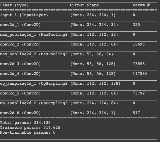
It’s finally time to train the model with Keras’ fit() function! The model trains for 300 epochs.
#Training
autoencoder_train = autoencoder.fit(train_X, train_ground, batch_size=batch_size,epochs=epochs,verbose=1,validation_data=(valid_X, valid_ground))
Finally! You trained the model on the fingerprint dataset for 300 epochs, Now, let’s plot the loss plot between training and validation data to visualize the model performance.
loss = autoencoder_train.history['loss']
val_loss = autoencoder_train.history['val_loss']
epochs = range(300)
plt.figure()
plt.plot(epochs, loss, 'bo', label='Training loss')
plt.plot(epochs, val_loss, 'b', label='Validation loss')
plt.title('Training and validation loss')
plt.legend()
plt.show()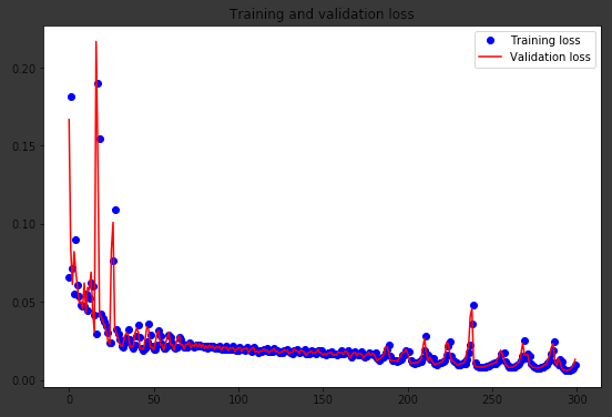
Finally, you can see that the validation loss and the training loss both are in sync. It shows that your model is not overfitting: the validation loss is decreasing and not increasing,
Therefore, you can say that your model’s generalization capability is good.
Finally, it’s time to reconstruct the test images using the predict() function of Keras and see how well your model is able to reconstruct the test data.
#Prediction
pred = autoencoder.predict(valid_X)#Reconstruction of Test Images
plt.figure(figsize=(20, 4))
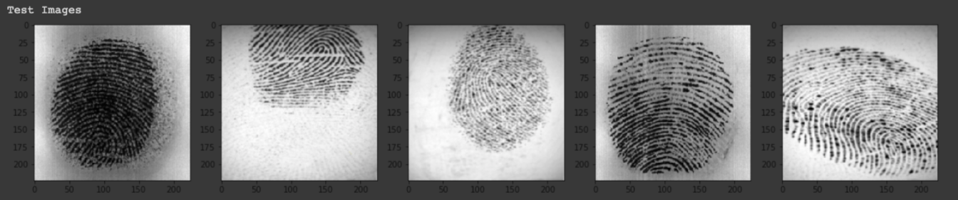
print("Test Images")
for i in range(5):
plt.subplot(1, 5, i+1)
plt.imshow(valid_ground[i, ..., 0], cmap='gray')
plt.show()
plt.figure(figsize=(20, 4))
print("Reconstruction of Test Images")
for i in range(5):
plt.subplot(1, 5, i+1)
plt.imshow(pred[i, ..., 0], cmap='gray')
plt.show()Test images:
Recreated images:

From the above figures, you can observe that your model did a fantastic job of reconstructing the test images that you predicted using the model. At least visually, the test and the reconstructed images look almost similar.
You can also find the code in my Github.
nageshsinghc4/Recreating-Fingerprints-using-Convolutional-Autoencoders
Build a Neural network that is capable of recreating or reconstructing fingerprint images. The dataset that I'm using…
Conclusion
It was never prevised that fingerprint science, which was used for catching criminals, would be used for unlocking mobile phones and authenticating payments. Phones instantly unlock when a finger registered with it, is put on the sensor, but it refuses to recognize the finger next to it, that’s when the uniqueness of fingerprints is practically felt.
Well, that’s all for this article hope you guys have enjoyed reading it and I’ll be glad if the article is of any help. Feel free to share your comments/thoughts/feedback in the comment section.
Thanks for reading!!!
Bio: Nagesh Singh Chauhan is a Big data developer at CirrusLabs. He has over 4 years of working experience in various sectors like Telecom, Analytics, Sales, Data Science having specialisation in various Big data components.
Original. Reposted with permission.
Related:
- Neural Networks 201: All About Autoencoders
- Stock Market Forecasting Using Time Series Analysis
- Exoplanet Hunting Using Machine Learning