 Linear to Logistic Regression, Explained Step by Step
 Linear to Logistic Regression, Explained Step by Step
Logistic Regression is a core supervised learning technique for solving classification problems. This article goes beyond its simple code to first understand the concepts behind the approach, and how it all emerges from the more basic technique of Linear Regression.
When we discuss solving classification problems, Logistic Regression should be the first supervised learning type algorithm that comes to our mind and is commonly used by many data scientists and statisticians. It is fundamental, powerful, and easy to implement. More importantly, its basic theoretical concepts are integral to understanding deep learning. So, I believe everyone who is passionate about machine learning should have acquired a strong foundation of Logistic Regression and theories behind the code on Scikit Learn. All right… Let’s start uncovering this mystery of Regression (the transformation from Simple Linear Regression to Logistic Regression)!
Linear Regression
I believe that everyone should have heard or even have learned about the Linear model in Mathethmics class at high school. Linear regression is the simplest and most extensively used statistical technique for predictive modelling analysis. It is a way to explain the relationship between a dependent variable (target) and one or more explanatory variables(predictors) using a straight line. There are two types of linear regression - Simple and Multiple.
Quick reminder: 4 Assumptions of Simple Linear Regression
- Linearity: The relationship between X and the mean of Y is linear.
- Homoscedasticity: The variance of residual is the same for any value of X (Constant variance of errors).
- Independence: Observations are independent of each other.
- Normality: The error(residuals) follow a normal distribution.
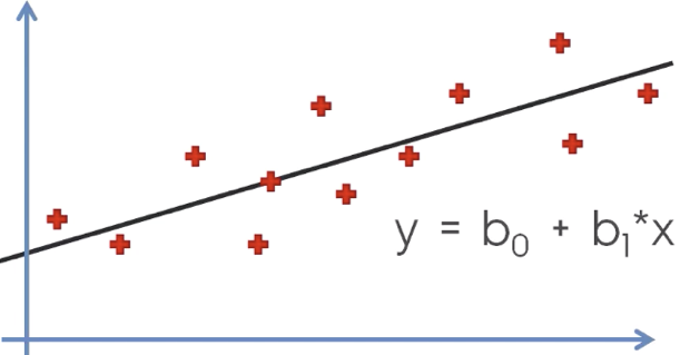
Simple Linear Regression with one explanatory variable (x): The red points are actual samples, we are able to find the black curve (y), all points can be connected using a (single) straight line with linear regression.
![]()
The equation of Multiple Linear Regression: X1, X2 … and Xn are explanatory variables.
You might have a question, “How to draw the straight line that fits as closely to these (sample) points as possible?” The most common method for fitting a regression line is the method of Ordinary Least Squares used to minimize the sum of squared errors (SSE) or mean squared error (MSE) between our observed value (yi) and our predicted value (ŷi).
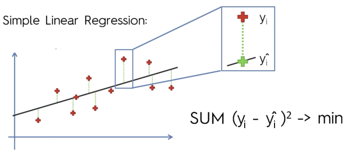
Residual: e = y — ŷ (Observed value — Predicted value).
From Numerical to Binary

Now we have a classification problem, and we want to predict the binary output variable Y (2 values: either 1 or 0). For example, the case of flipping a coin (Head/Tail). The response yi is binary: 1 if the coin is Head, 0 if the coin is Tail. This is represented by a Bernoulli variable where the probabilities are bounded on both ends (they must be between 0 and 1).

The linear regression line is below 0.
Linear regression is only dealing with continuous variables instead of Bernoulli variables. The problem of Linear Regression is that these predictions are not sensible for classification since the true probability must fall between 0 and 1, but it can be larger than 1 or smaller than 0. Noted that classification is not normally distributed which is violated assumption 4: Normality. Moreover, both mean and variance depend on the underlying probability. Any factor that affects the probability will change not just the mean but also the variance of the observations, which means the variance is no longer constantly violating the assumption 2: Homoscedasticity. As a result, we cannot directly apply linear regression because it won't be a good fit.
So…how can we predict a classification problem?
Instead, we can transform our linear regression to a logistic regression curve!
As we are now looking for a model for probabilities, we should ensure the model predicts values on the scale from 0 to 1. A powerful model Generalised linear model (GLM) caters to these situations by allowing for response variables that have arbitrary distributions (other than only normal distributions), and by using a link function to vary linearly with the predicted values rather than assuming that the response itself must vary linearly with the predictor. As a result, GLM offers extra flexibility in modelling. In this case, we need to apply the logistic function (also called the ‘inverse logit’ or ‘sigmoid function’).
Logistic Regression is a type of Generalized Linear Models.
Before we dig deep into logistic regression, we need to clear up some of the fundamentals of statistical terms — Probability and Odds.
The probability that an event will occur is the fraction of times you expect to see that event in many trials. If the probability of an event occurring is Y, then the probability of the event not occurring is 1-Y. Probabilities always range between 0 and 1.
The odds are defined as the probability that the event will occur divided by the probability that the event will not occur. Unlike probability, the odds are not constrained to lie between 0 and 1 but can take any value from zero to infinity.
If the probability of Success is P, then the odds of that event is:
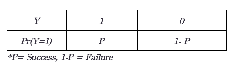
Odds: Success/ Failure.
Example: If the probability of success (P) is 0.60 (60%), then the probability of failure(1-P) is 1–0.60 = 0.40(40%). Then the odds are 0.60 / (1–0.60) = 0.60/0.40 = 1.5.
It’s time… to transform the model from linear regression to logistic regression using the logistic function.

In (odd)=bo+b1x
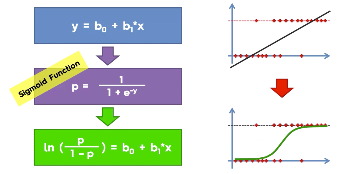
logistic function (also called the ‘inverse logit’).
We can see from the below figure that the output of the linear regression is passed through a sigmoid function (logit function) that can map any real value between 0 and 1.
Logistic Regression is all about predicting binary variables, not predicting continuous variables.
Don’t get confused with the term ‘Regression’ presented in Logistic Regression. I know it’s pretty confusing, for the previous ‘me’ as well :D
Congrats~you have gone through all the theoretical concepts of the regression model. Feel bored?! Here’s a real case to get your hands dirty!
Imagine that you are a store manager at the APPLE store, increasing 10% of the sales revenue is your goal this month. Therefore, you need to know who the potential customers are in order to maximise the sale amount.

Image from Apple.
The client information you have is including Estimated Salary, Gender, Age, and Customer ID.
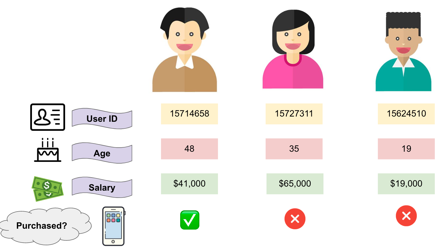
3 samples of client information.
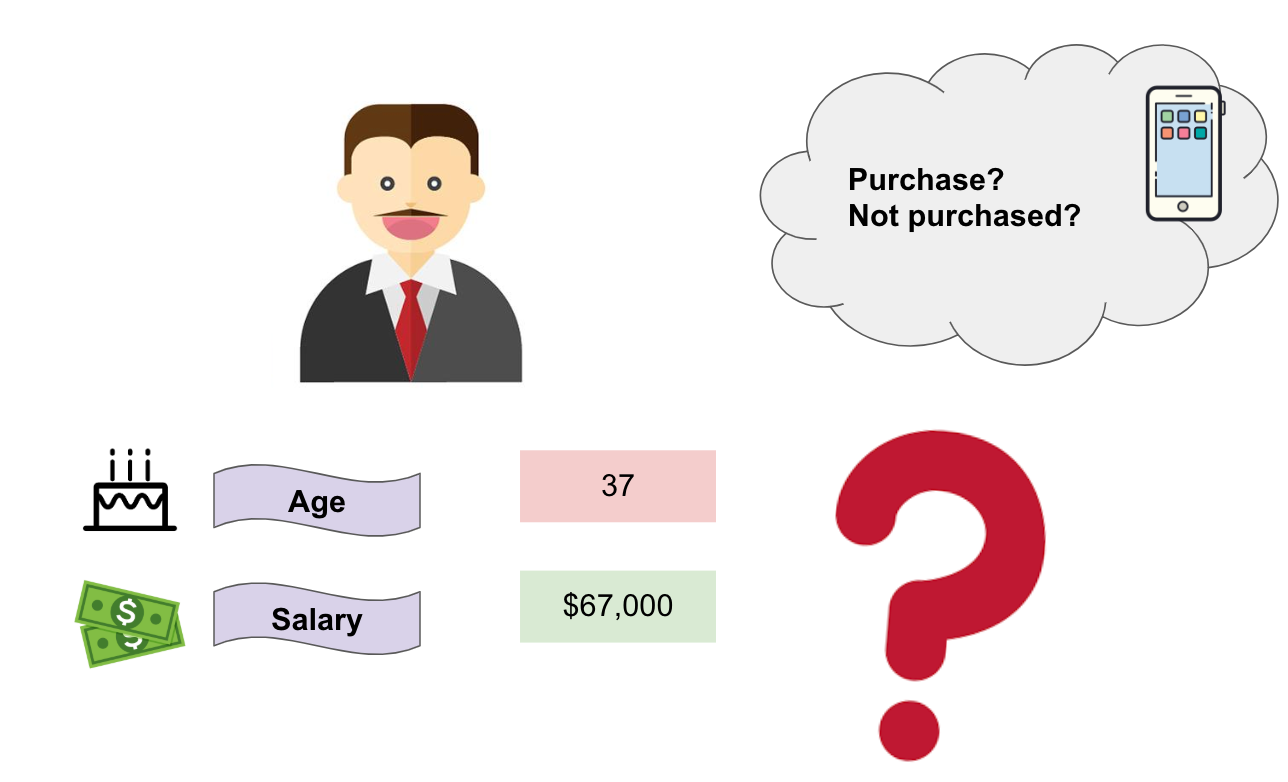
If now we have a new potential client who is 37 years old and earns $67,000, can we predict whether he will purchase an iPhone or not (Purchase?/ Not purchase?)
Coding Time: Let’s build a logistic regression model with Scikit-learn to predict who the potential clients are together!
# import the libraries
import numpy as np
import pandas as pd
# import the dataset
dataset = pd.read_csv('Social_Network_Ads.csv')
# get dummy variables
df_getdummy=pd.get_dummies(data=df, columns=['Gender'])
# seperate X and y variables
X = df_getdummy.drop('Purchased',axis=1)
y = df_getdummy['Purchased']
# split the dataset into the Training set and Test set
from sklearn.model_selection import train_test_split
X_train, X_test, y_train, y_test = train_test_split(X, y, test_size = 0.25, random_state = 0)
# feature scaling
from sklearn.preprocessing import StandardScaler
sc = StandardScaler()
X_train = sc.fit_transform(X_train)
X_test = sc.transform(X_test)
# fit Logistic Regression to the training set
from sklearn.linear_model import LogisticRegression
classifier = LogisticRegression(random_state = 0)
classifier.fit(X_train, y_train)
# predict the Test set results
y_pred = classifier.predict(X_test)
# make the confusion matrix for evaluation
from sklearn.metrics import confusion_matrix
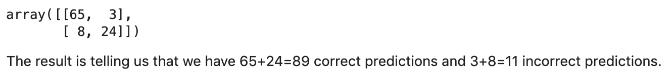
confusion_matrix(y_test, predictions)
Output
# find accuracy socre (Accuracy = number of times you’re right / number of predictions)

from sklearn.metrics import accuracy_score
accuracy_score(y_true=y_train, y_pred=LogReg_model.predict(X_train))
Output
0.8333333333333334
The accuracy is 83%
For the coding and dataset, please check out here.
Summary
- The limitations of linear regression
- The understanding of “Odd” and “Probability”
- The transformation from linear to logistic regression
- How logistic regression can solve the classification problems in Python
Original. Reposted with permission.
Related: