Hyperparameter Optimization for Machine Learning Models

Credits

Introduction

 
Model optimization is one of the toughest challenges in the implementation of machine learning solutions. Entire branches of machine learning and deep learning theory have been dedicated to the optimization of models.

Hyperparameter optimization in machine learning intends to find the hyperparameters of a given machine learning algorithm that deliver the best performance as measured on a validation set. Hyperparameters, in contrast to model parameters, are set by the machine learning engineer before training. The number of trees in a random forest is a hyperparameter while the weights in a neural network are model parameters learned during training. I like to think of hyperparameters as the model settings to be tuned so that the model can optimally solve the machine learning problem.

Some examples of model hyperparameters include:

• The learning rate for training a neural network.
• The C and ???? hyperparameters for support vector machines.
• The k in k-nearest neighbors.

Hyperparameter optimization finds a combination of hyperparameters that returns an optimal model which reduces a predefined loss function and in turn increases the accuracy on given independent data.

Classification models with their respective hyperparameters.

Hyperparameter Optimization methods

 
Hyperparameters can have a direct impact on the training of machine learning algorithms. Thus, to achieve maximal performance, it is important to understand how to optimize them. Here are some common strategies for optimizing hyperparameters:

1. Manual Hyperparameter Tuning

 
Traditionally, hyperparameters were tuned manually by trial and error. This is still commonly done, and experienced engineers can “guess” parameter values that will deliver very high accuracy for ML models. However, there is a continual search for better, faster, and more automatic methods to optimize hyperparameters.

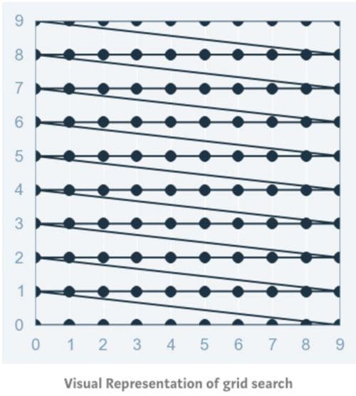
2. Grid Search

 
Grid search is arguably the most basic hyperparameter tuning method. With this technique, we simply build a model for each possible combination of all of the hyperparameter values provided, evaluating each model, and selecting the architecture which produces the best results.

Grid-search does NOT only apply to one model type but can be applied across machine learning to calculate the best parameters to use for any given model.

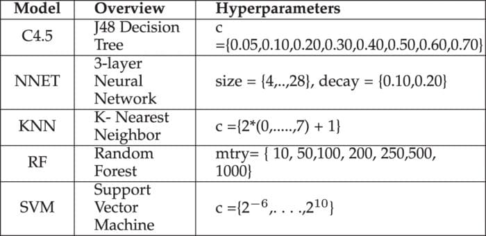
For example, a typical soft-margin SVM classifier equipped with an RBF kernel has at least two hyperparameters that need to be optimized for good performance on unseen data: a regularization constant C and a kernel hyperparameter γ. Both parameters are continuous, so to perform grid search, one selects a finite set of “reasonable” values for each, let’s say

Grid search then trains an SVM with each pair (C, γ) in the cartesian product of these two sets and evaluates their performance on a held-out validation set (or by internal cross-validation on the training set, in which case multiple SVMs are trained per pair). Finally, the grid search algorithm outputs the settings that achieved the highest score in the validation procedure.
How does it work in python?

from sklearn.datasets import load_iris
from sklearn.svm import SVC
iris = load_iris()
svc = SVR()

Here’s a python implementation of grid search using GridSearchCV from the sklearn library.

from sklearn.model_selection import GridSearchCV
from sklearn.svm import SVR
grid = GridSearchCV(
        estimator=SVR(kernel='rbf'),
        param_grid={
            'C': [0.1, 1, 100, 1000],
            'epsilon': [0.0001, 0.0005, 0.001, 0.005, 0.01, 0.05, 0.1, 0.5, 1, 5, 10],
            'gamma': [0.0001, 0.001, 0.005, 0.1, 1, 3, 5]
        },
        cv=5, scoring='neg_mean_squared_error', verbose=0, n_jobs=-1)

Fitting the Grid Search:

grid.fit(X,y)

Methods to Run on Grid-Search:

#print the best score throughout the grid search
print grid.best_score_#print the best parameter used for the highest score of the model.
print grid.best_param_

We then use the best set of hyperparameter values chosen in the grid search, in the actual model as shown above.

One of the drawbacks of grid search is that when it comes to dimensionality, it suffers when evaluating the number of hyperparameters grows exponentially. However, there is no guarantee that the search will produce the perfect solution, as it usually finds one by aliasing around the right set.

3. Random Search

 
Often some of the hyperparameters matter much more than others. Performing random search rather than grid search allows a much more precise discovery of good values for the important ones.

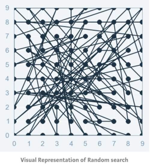
Random Search sets up a grid of hyperparameter values and selects random combinations to train the model and score. This allows you to explicitly control the number of parameter combinations that are attempted. The number of search iterations is set based on time or resources. Scikit Learn offers the RandomizedSearchCV function for this process.

While it’s possible that RandomizedSearchCV will not find as accurate a result as GridSearchCV, it surprisingly picks the best result more often than not and in a fraction of the time it takes GridSearchCV would have taken. Given the same resources, Randomized Search can even outperform Grid Search. This can be visualized in the graphic below when continuous parameters are used.

The chances of finding the optimal parameter are comparatively higher in random search because of the random search pattern where the model might end up being trained on the optimized parameters without any aliasing. Random search works best for lower dimensional data since the time taken to find the right set is less with less number of iterations. Random search is the best parameter search technique when there is less number of dimensions.

In the case of deep learning algorithms, it outperforms the grid search.

Credits

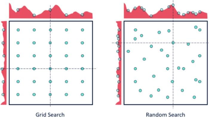
In the above figure, yay that you have two parameters, with 5x6 grid search you check only 5 different parameter values from each of the parameters (six rows and five columns on the plot on the left), while with the random search you check 14 different parameter values of each of the parameters.

How does it work in python?

from sklearn.datasets import load_iris
from sklearn.ensemble import RandomForestRegressor
iris = load_iris()
rf = RandomForestRegressor(random_state = 42)

Here’s a python implementation of grid search using RandomizedSearchCV of the sklearn library.

from sklearn.model_selection import RandomizedSearchCV
random_grid = {'n_estimators': n_estimators,
               'max_features': max_features,
               'max_depth': max_depth,
               'min_samples_split': min_samples_split,
               'min_samples_leaf': min_samples_leaf,
               'bootstrap': bootstrap}rf_random = RandomizedSearchCV(estimator = rf, param_distributions = random_grid, n_iter = 100, cv = 3, verbose=2, random_state=42, n_jobs = -1)# Fit the random search model

Fitting the Random Search:

rf_random.fit(X,y)

Methods to Run on Grid-Search:

#print the best score throughout the grid search
print rf_random.best_score_#print the best parameter used for the highest score of the model.
print rf_random.best_param_Output:
{'bootstrap': True,
 'max_depth': 70,
 'max_features': 'auto',
 'min_samples_leaf': 4,
 'min_samples_split': 10,
 'n_estimators': 400}

4. Bayesian Optimization

 
The previous two methods performed individual experiments building models with various hyperparameter values and recording the model performance for each. Because each experiment was performed in isolation, it’s very easy to parallelize this process. However, because each experiment was performed in isolation, we’re not able to use the information from one experiment to improve the next experiment. Bayesian optimization belongs to a class of sequential model-based optimization (SMBO) algorithms that allow for one to use the results of our previous iteration to improve our sampling method of the next experiment.

This, in turn, limits the number of times a model needs to be trained for validation as solely those settings that are expected to generate a higher validation score are passed through for evaluation.

Bayesian optimization works by constructing a posterior distribution of functions (Gaussian process) that best describes the function you want to optimize. As the number of observations grows, the posterior distribution improves, and the algorithm becomes more certain of which regions in parameter space are worth exploring and which are not.

We can see this in the image below:

Source: bayesian-optimization

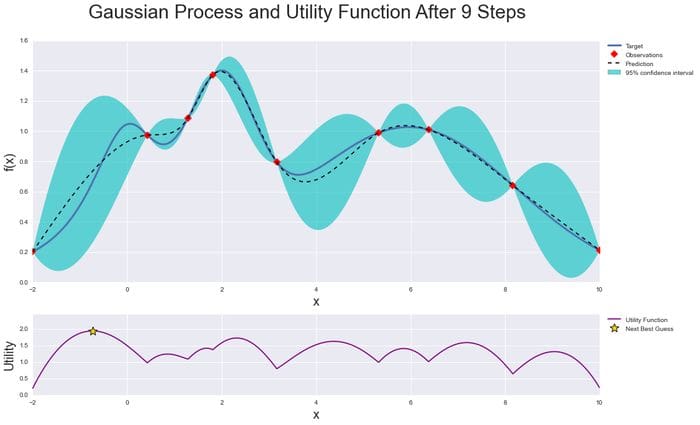
As you iterate over and over, the algorithm balances its needs of exploration and exploitation taking into account what it knows about the target function. At each step, a Gaussian Process is fitted to the known samples (points previously explored), and the posterior distribution, combined with an exploration strategy (such as UCB (Upper Confidence Bound), or EI (Expected Improvement)), is used to determine the next point that should be explored.

Using Bayesian Optimization, we can explore the parameter space more smartly, and thus reduce the time required to do this process.

You can check the python implementation of Bayesian optimization below:

thuijskens/bayesian-optimization

5. Gradient-based Optimization

 
It is specially used in the case of Neural Networks. It computes the gradient with respect to hyperparameters and optimizes them using the gradient descent algorithm.

The calculation of the gradient is the least of problems. At least in times of advanced automatic differentiation software. (Implementing this in a general way for all sklearn-classifiers, of course, is not easy).

Credits

And while there are works of people who used this kind of idea, they only did this for some specific and well-formulated problem (e.g. SVM-tuning). Furthermore, there probably were a lot of assumptions because:

Why is this not a good idea?

1. Hyperparameter optimization is in general non-smooth

• GD really likes smooth functions as a gradient of zero is not helpful
• Each hyper-parameter which is defined by some discrete-set (e.g. choice of l1 vs. l2 penalization) introduces non-smooth surfaces.

2. Hyperparameter optimization is in general non-convex

• The whole convergence-theory of gradient descent assumes, that the underlying problem is convex.
• Good-case: you obtain some local-minimum (can be arbitrarily bad).
• Worst-case: gradient descent is not even converging to some local-minimum.

To get python implementation and more about the Gradient Descent Optimization algorithm click here.

6. Evolutionary Optimization

 
Evolutionary optimization follows a process inspired by the biological concept of evolution and since natural evolution is a dynamic process in a changing environment, they are also well suited to dynamic optimization problems.

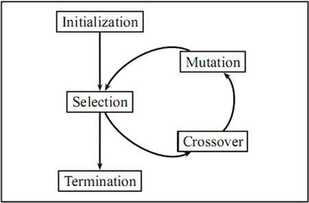
Evolutionary algorithms are often used to find good approximate solutions that cannot be easily solved by other techniques. Optimization problems often don’t have an exact solution as it may be too time-consuming and computationally intensive to find an optimal solution. However, evolutionary algorithms are ideal in such situations as they can be used to find a near-optimal solution which is often sufficient.

One advantage of evolutionary algorithms is that they develop solutions free of any human misconceptions or biases, which means they can produce surprising ideas which we might never generate ourselves.

You can learn more about evolutionary algorithms here. You can also check python implementation here.

As a general rule of thumb, any time you want to optimize tuning hyperparameters, think Grid Search and Randomized Search!

Conclusion

 
In this article, we’ve learned that finding the right values for hyperparameters can be a frustrating task and can lead to underfitting or overfitting machine learning models. We saw how this hurdle can be overcome by using Grid Search & Randomized Search and other algorithms — which optimize tuning of hyperparameters to save time and eliminate the chance of overfitting or underfitting by random guessing.

Well, this concludes this article. I hope you guys have enjoyed reading it, feel free to share your comments/thoughts/feedback in the comment section.

Thanks for reading !!!

 
Bio: Nagesh Singh Chauhan is a Data Science enthusiast. Interested in Big Data, Python, Machine Learning.

Original. Reposted with permission.

Related:

• How to Do Hyperparameter Tuning on Any Python Script in 3 Easy Steps
• Coronavirus COVID-19 Genome Analysis using Biopython
• Practical Hyperparameter Optimization