How Do Neural Networks Learn?

By Dorian Lazar, Writer, Towards AI.

Photo by Jason Leung on Unsplash.

Neural networks are, without a doubt, the most popular machine learning technique that is used nowadays. So, I think it is worth understanding how they actually learn.

To do so, let us first take a look at the image below:

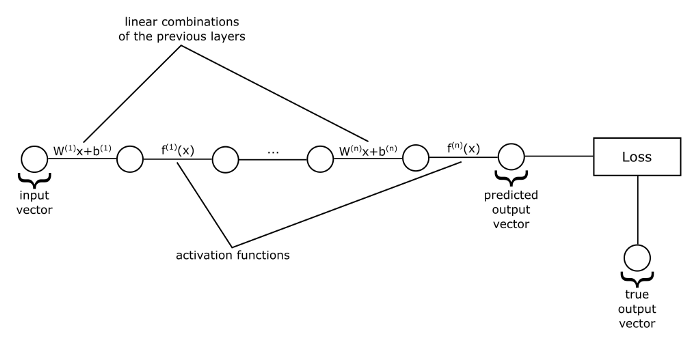
If we represent the input and output values of each layer as vectors, the weights as matrices, and biases as vectors, then we get the above-flattened view of a neural network which is just a sequence of vector function applications. That is, functions that take vectors as input, do some transformation on them, and they output other vectors. In the image above, each line represents a function, which can be either a matrix multiplication plus a bias vector, or an activation function. And the circles represent the vectors on which these functions operate.

For example, we start with the input vector, and then we feed it into the first function, which computes linear combinations of its components, then we obtain another vector as output. This last vector we feed as input to the activation function, and so on until we get to the last function in our sequence. The output of this last function will be the predicted value of our network.

We have discussed so far how a neural network gets its output, which we are interested in, it just passes its input vector through a sequence of functions. But these functions depend on some parameters: the weights and biases.

How do we actually learn those parameters in order to obtain good predictions?

Well, let us recall what a neural network actually is: it is just a function, a big function composed of smaller ones that are applied in sequence. This function has a set of parameters that, because at first, we have no idea what they should be, we just initialize them randomly. So, at first, our network will give us just random values. How can we improve them? Before attempting to improve them, we first need a way of evaluating the performance of our network. How are we supposed to improve the performance of our model if we do not have a way to measure how good or how bad is it doing?

For that, we need to come up with a function that takes as input the predictions of our network and the true labels in our dataset, and to give us a number that represents the performance of our network. Then we can turn the learning problem into an optimization problem of finding the minimum or maximum of this function. In the machine learning community, this function usually measures how bad our predictions are, hence it is named a loss function. And our problem is to find the parameters of our network that minimizes this loss function.

 

Stochastic gradient descent

 

You may be familiar with the problem of finding the minimum of a function from your calculus class. There you usually take the gradient of your function, set it equal to 0, find all the solutions (also called critical points), and then choose among them the one that gives your function the smallest value. And that is the global minimum. Can we do the same thing in minimizing our loss function? Not really. The problem is that the loss function of a neural network is not as nice and compact as those you usually find in calculus textbooks. It is an extremely complicated function with thousands, hundreds of thousands, or even millions of parameters. It may be even impossible to find a closed-form solution to this problem. This problem is usually approached by iterative methods, methods that do not try to find a direct solution, but instead, they start with a random solution and try to improve it a little bit in each iteration. Eventually, after a large number of iterations, we will get a rather good solution.

One such iterative method is gradient descent. As you may know, the gradient of a function gives us the direction of the steepest ascent. If we take the negative of the gradient, it will give us the direction of the steepest descent, that is the direction in which we can get the fastest towards a minimum. So, at each iteration, also called an epoch, we compute the gradient of the loss function and subtract it (multiplied by a factor called learning rate) from the old parameters to get the new parameters of our network.

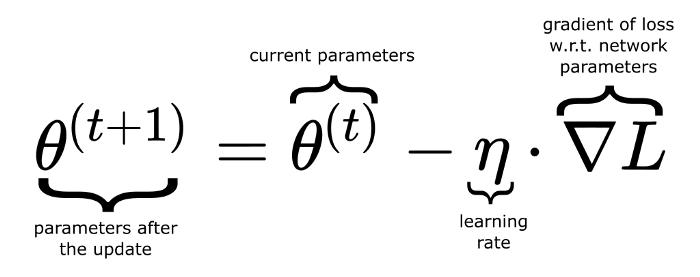
Here, θ (theta) represents a vector containing all the network’s parameters.

In the standard gradient descent method, the gradient is computed considering the whole dataset. Usually, this is not desirable as it may be computationally expensive. In practice, the dataset is randomly divided into more chunks called batches, and an update is made for each one of these batches. This is called stochastic gradient descent.

The above update rule considers at each step only the gradient evaluated at the current position. In this way, the trajectory of the point that moves on the surface of the loss function is sensitive to any perturbation. Sometimes we may want to make this trajectory more robust. For that, we use a concept inspired from physics: momentum. The idea is that when we do the update to also take into consideration previous updates, that accumulates into a variable Δθ. If more updates are done in the same direction, then we will go “faster” into that direction and will not change our trajectory by any small perturbation. Think about this like velocity.

Here, α is a non-negative factor that determines the contribution of past gradients. When it is 0, we simply do not use momentum.

 

Backpropagation

 

How do we actually compute the gradient? Recall that a neural network, and thus the loss function, is just a composition of functions. How can we compute partial derivatives of composite functions? Using the chain rule. Let us look at the following image:

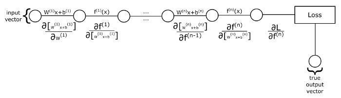
If we want to compute the partial derivatives of the loss w.r.t. (with respect to) the weights of the first layer, then we take the derivative of the first linear combination w.r.t. the weights, then we multiply with the derivative of the next function (the activation function) w.r.t. the output from the previous function, and so on until we multiply with the derivative of the loss w.r.t. the last activation function. What if we want to compute the derivative w.r.t. the weights of the second layer? We have to do the same process, but this time we start with the derivative of the second linear combination function w.r.t. its weights, and after that, the rest of the terms that we have to multiply with were also present when we computed the derivative of the weights of the first layer. So, instead of computing these terms over and over again, we will go backward, hence the name backpropagation.

We will first start by computing the derivative of the loss w.r.t. the output of our network, and then propagate these derivatives backwards towards the first layer by maintaining a running product of derivatives. Note that there are 2 kinds of derivatives that we take: one in which we compute the derivative of a function w.r.t. its input. These we multiply to our product of derivatives and have the purpose of keeping track of the error of the network from its output to the current point in which we are in the algorithm. The second kind of derivatives is one that we take w.r.t. the parameters that we want to optimize. These we do not multiply with the rest of our product of derivatives. Instead, we store them as part of the gradient that we will use later to update the parameters.

So, while backpropagation, when we encounter functions that do not have learnable parameters (like activation functions), we take derivatives only of the first kind, just to propagate the errors backwards. But, when we encounter functions that do have learnable parameters (like the linear combinations, where we have the weights and biases that we want to learn) we take derivatives of both kinds: the first one w.r.t. its input for error propagation, and the second one w.r.t. its weights and biases, and store them as part of the gradient. We do this process starting from the loss function and until we get to the first layer where we do not have any learnable parameters that we want to add to the gradient. This is the backpropagation algorithm.

 

Softmax activation & Cross-entropy loss

 

A commonly used activation function for the last layer in a classification task is the softmax function.

The softmax function transforms its input vector into a probability distribution. If you look above, you can see that the elements of the softmax’s output vector have the properties that they are all positive, and their sum is 1. When we use softmax activation, we create in the last layer as many nodes as the number of classes in our dataset, and the softmax activation will give us a probability distribution over the possible classes. So, the output of the network will give us the probability that the input vector belongs to each one of the possible classes, and we choose the class that has the highest probability and reports that as the prediction of our network.

When softmax is used as the activation of the output layer, we usually use as loss function the cross-entropy loss. The cross-entropy loss measures how similar are 2 probability distributions. We can represent the true label of our input x as a probability distribution: one in which we have a probability of 1 for the true class label and 0 for the other class labels. This representation of labels is also called one-hot encoding. Then we use cross-entropy to measure how close is the predicted probability distribution of our network to the true one.

Where y is the one-hot encoding of the true label, y hat is the predicted probability distribution, and yi, yi hat are elements of those vectors.

If the predicted probability distribution is close to the one-hot encoding of the true labels, then the loss would be close to 0. Otherwise, if they are hugely different, the loss can potentially grow to infinity.

 

Mean squared error loss

 

The softmax activation and cross-entropy loss are mainly for classification tasks, but neural networks can easily be adapted to regression tasks by just using an appropriate loss function and activation in the last layer. For example, if instead of class labels as ground truth, we have a list of numbers that we want to approximate we can use mean squared error (MSE for short) loss. Usually, when we use MSE loss, we use the identity activation (that is, f(x) = x) in the last layer.

To conclude, the learning process of a neural network is nothing more than just an optimization problem: we want to find the parameters that minimize a loss function. But that is not an easy task, and there are whole books written about optimization techniques. And, besides optimization, there also arise problems about which neural network architecture to choose for a given task.

Original. Reposted with permission.

 

Related:

• Learning by Forgetting: Deep Neural Networks and the Jennifer Aniston Neuron
• Introduction to Convolutional Neural Networks
• 5 Concepts You Should Know About Gradient Descent and Cost Function