Introduction to Convolutional Neural Networks

 

Have you ever thought how facial recognition works on social media, or how object detection helps in building self-driving cars, or how disease detection is done using visual imagery in healthcare? It’s all possible thanks to convolutional neural networks (CNN).

 

Introduction

 
Just like how a child learns to recognize objects, we need to show an algorithm, millions of pictures before it can generalize the input and make predictions for images it has never seen before.

Computers ‘see’ in a different way than we do. Their world consists of only numbers. Every image can be represented as 2-dimensional arrays of numbers, known as pixels.

 

But the fact that they perceive images differently, doesn’t mean we can’t train them to recognize patterns as we do. We just have to think of what an image is different.

To teach an algorithm on how to recognize objects in images, we use a specific type of Artificial Neural Network: a Convolutional Neural Network (CNN). Their name stems from one of the most important operations in the network called convolution.

 

Convolutional Neural Networks

 
Convolutional Neural Networks(CNN or ConvNets) are ordinary neural networks that assume that the inputs are image. They are used to analyze and classify images, cluster images by similarity, and perform object recognition within a frame. For example, convolutional neural networks (ConvNets or CNNs) are used to identify faces, individuals, street signs, tumors, platypuses, and many other aspects of visual data.

 

Biological connection of CNN

 
When you first heard of the term convolutional neural networks, you may have thought of something related to neuroscience or biology, and you would be right. Sort of. CNN’s do take a biological inspiration from the visual cortex. The visual cortex has small regions of cells that are sensitive to specific regions of the visual field.

This idea was expanded upon by a fascinating experiment by Hubel and Wiesel in 1962 (Video) where they showed that some individual neuronal cells in the brain responded (or fired) only in the presence of edges of a certain orientation. For example, some neurons fired when exposed to vertical edges and some when shown horizontal or diagonal edges. Hubel and Wiesel found out that all of these neurons were organized in a columnar architecture and that together, they were able to produce visual perception. This idea of specialized components inside of a system having specific tasks (the neuronal cells in the visual cortex looking for specific characteristics) is one that machines use as well and is the basis behind CNNs.

Before you move ahead I would strongly recommend checking the below article to have a basic understanding of Neural Networks if you are a beginner in deep learning.

Introduction to Artificial Neural Networks
 

 

How Convolutional Neural Networks learn?

 
Images are made up of pixels. Each pixel is represented by a number between 0 and 255. Therefore each image has a digital representation which is how computers can work with images.

There are 4 major operations in CNN image detection/classification.

1. Convolution
2. Activation map
3. Max pooling
4. Flattening
5. Fully connected layer

 

1.1 Convolution

 
Convolution operation works on 2 signals in 1D and 2 images in 2D. Mathematically a convolution is a combined integration of two functions that shows you how one function modifies the other:

The main purpose of a convolutional layer is to detect features or visual features in images such as edges, lines, color drops, etc. This is a very interesting property because, once it has learned a characteristic at a specific point in the image, it can recognize it later in any part of it.

CNN’s make use of filters (also known as kernels, feature detectors), to detect features, such as edges, are present throughout an image. A filter is just a matrix of values, called weights, that are trained to detect specific features. The filter moves over each part of the image to check if the feature it is meant to detect is present. To provide a value representing how confident it is that a specific feature is present, the filter carries out a convolution operation, which is an element-wise product and sum between two matrices.

When the feature is present in part of an image, the convolution operation between the filter and that part of the image results in a real number with a high value. If the feature is not present, the resulting value is low.

In the below image a filter that is trained for detecting plus sign is passed over a part of the image. Since that part of the image contains the same plus that the filter is looking for, the result of the convolution operation is a large number.

Convolution(element-wise product and sum) = (50*50)+(50*50)+(50*50)+(50*50)+(50*50)+(60*60)+(60*60)+(40*50)+(40*50)+(50*50)+(50*50)+(40*50)+(50*50)+(50*50) = Very large real number

But when that same filter/kernel is passed over a part of the image with a considerably different set of edges, the convolution’s output is small, meaning that there was no strong presence of any plus sign and element-wise product and sum will result in zero or very less value.

So we need N number of feature detectors to detect different curves/edges of the image.

 

The result of passing this filter over the entire image is an output matrix called feature maps or convolved features that stores the convolutions of this filter over various parts of the image. Now since we have multiple filters, we end up with a 3D output: one 2D feature map per filter. The filter must have the same number of channels as the input image so that the element-wise multiplication can take place.

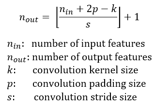
Additionally, a filter can be slid over the input image at varying intervals, using a stride value. The stride value dictates by how much the filter should move at each step.

 

We can determine the number of output layers of a given convolutional block:

 

1.2 Padding

 
One tricky issue when applying convolutional layers is that we tend to lose pixels on the perimeter of our image. Since we typically use small kernels, for any given convolution, we might only lose a few pixels, but this can add up as we apply many successive convolutional layers.

Padding refers to the number of pixels added to an image when it is being processed by the kernel of a CNN.

One solution to assist the kernel with processing the image, pad the image with zeros(zero-padding) to allow for more space for the kernel to cover the image. Adding padding to an image processed by a CNN allows for a more accurate analysis of images.

 

 

2.1 Activation Map

 
These feature maps must be passed through a non-linear mapping. The feature maps are summed with a bias term and passed through a non-linear activation function: ReLu. The purpose of the activation function is to introduce non-linearity into our network because the images are made of different objects that are not linear to each other so the images are highly non-linear.

 

2.2 Max Pooling

 
After ReLU comes to a pooling step, in which the CNN downsamples the convolved feature (to save on processing time), while also reducing the size of the image. This helps reduce overfitting, which would occur if CNN is given too much information, especially if that information is not relevant in classifying the image.

There are different types of pooling, for example, max pooling and min pooling. In max pooling, a window passes over an image according to a set stride value. At each step, the maximum value within the window is pooled into an output matrix, hence the name max pooling.

These values then form a new matrix called a pooled feature map.

An added benefit of max-pooling is that it forces the network to focus on a few neurons instead of all of them which has a regularizing effect on the network, making it less likely to overfit the training data and hopefully generalize well.

 

3.3 Flattening

 
After multiple convolution layers and downsampling operations, the 3D representation of the image is converted into a feature vector that is passed into a multi-layer perceptron to output probabilities. The following image describes the flattening operation:

 

The rows are concatenated to form a long feature vector. If multiple input layers are present, its rows are also concatenated to form an even longer feature vector.

 

4. Fully Connected Layer

 
In this step, the flattened feature map is passed through a neural network. This step is made up of the input layer, the fully connected layer, and the output layer. The fully connected layer is similar to the hidden layer in ANNs but in this case, it’s fully connected. The output layer is where we get the predicted classes. The information is passed through the network and the error of prediction is calculated. The error is then backpropagated through the system to improve the prediction.

 

The final output produced by the dense layer neural network doesn’t usually add up to one. However, these outputs must be brought down to numbers between zero and one, which represent the probability of each class. This is the role of the Softmax function.

The output of this dense layer is therefore passed through the Softmax activation function, which maps all the final dense layer outputs to a vector whose elements sum up to one:

 

The way this fully connected layer works is that it looks at the output of the previous layer (which as we remember should represent the activation maps of high-level features) and determines which features most correlate to a particular class. For example, if the program is predicting that some image is a dog, it will have high values in the activation maps that represent high-level features like a paw or 4 legs, etc. Similarly, if the program is predicting that some image is a bird, it will have high values in the activation maps that represent high-level features like wings or a beak, etc. A Fully Connected layer looks at what high level features most strongly correlate to a particular class and has particular weights so that when you compute the products between the weights and the previous layer, you get the correct probabilities for the different classes.

Let’s summarize to see the entire process about how CNN recognizes:

• The pixels from the image are fed to the convolutional layer that performs the convolution operation
• It results in a convolved map
• The convolved map is applied to a ReLU function to generate a rectified feature map
• The image is processed with multiple convolutions and ReLU layers for locating the features
• Different pooling layers with various filters are used to identify specific parts of the image
• The pooled feature map is flattened and fed to a fully connected layer to get the final output

 

CNN Implementation with Keras

 
Now let’s write the code that can classify images. This code can be applied with most image datasets available with little modification. So once you have your image data, separate them into folders and give them their appropriate names, i.e the training set and the test set.

 

Building the CNN

 
In this step, the first step is to build the Convolutional Neural Network with below-mentioned layers:

• Sequential is used to initialize the neural network.
• Convolution2D is used to make the convolutional network that deals with the images.
• MaxPooling2D layer is used to add the pooling layers.
• Flatten is the function that converts the pooled feature map to a single column that is passed to the fully connected layer.
• Dense adds the fully connected layer to the neural network.

Once the network is built, then compile/train the network using Stochastic Gradient Descent(SGD). Gradient Descent works fine when we have a convex curve. But if we don’t have a convex curve, Gradient Descent fails. Hence, in Stochastic Gradient Descent, few samples are selected randomly instead of the whole data set for each iteration.

Now since the network is compiled, its time to train the CNN model with the training images.

Fitting the CNN to the images

Perform Image Augmentation instead of training your model with lots of images we can train our model with fewer images and training the model with different angles and modifying the images. Keras has this ImageDataGenerator class which allows the users to perform image augmentation on the fly in a very easy way.

Once you have trained your CNN network with the training image dataset, its time to check the accuracy of your model.

 

Conclusion

 
CNN is the best artificial neural network, it is used for modeling image but it is not limited to just modeling of the image but out of many of its applications. There are many improvised versions based on CNN architecture like AlexNet, VGG, YOLO, and many more.
Well, that’s all for this article hope you guys have enjoyed reading it and I’ll be glad if the article is of any help. Feel free to share your comments/thoughts/feedback in the comment section.

Thanks for reading!!!

 
Bio: Nagesh Singh Chauhan is a Big data developer at CirrusLabs. He has over 4 years of working experience in various sectors like Telecom, Analytics, Sales, Data Science having specialisation in various Big data components.

Original. Reposted with permission.

Related:

• 5 Papers on CNNs Every Data Scientist Should Read
• Model Evaluation Metrics in Machine Learning
• Dimensionality Reduction with Principal Component Analysis (PCA)