Every Complex DataFrame Manipulation, Explained & Visualized Intuitively

By Andre Ye, Cofounder at Critiq, Editor & Top Writer at Medium.

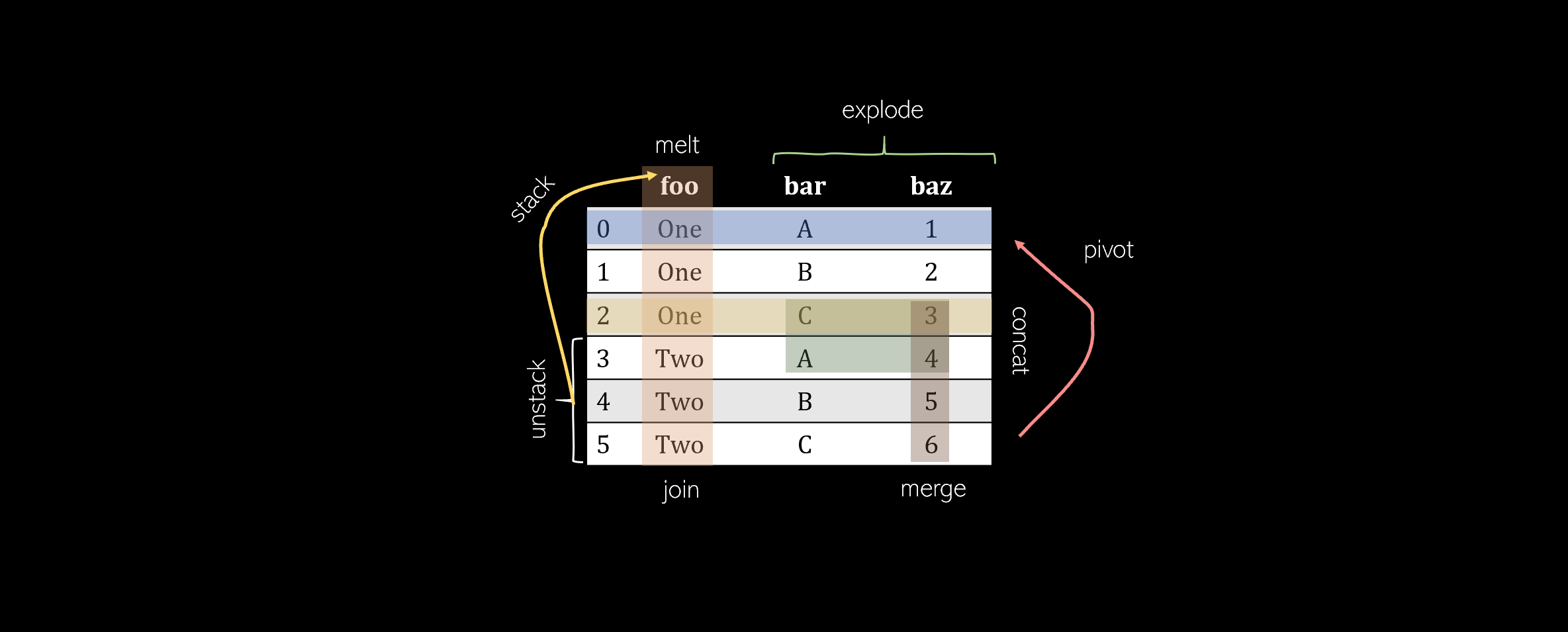
Pandas offers a wide range of DataFrame manipulations, but many of them are complex and may not seem approachable. This article presents 8 essential DataFrame manipulation methods that cover almost all of the manipulation functions a data scientist would need to know. Each method will include an explanation, visualization, code, and tricks to remember it.

Pivot

Pivoting a table creates a new ‘pivoted table’ that projects existing columns in the data as elements of a new table, being the index, column, and the values. The columns in the initial DataFrame that will become the index and the columns are displayed as unique values, and combinations of these two columns will be displayed as the value. This means that pivots cannot handle duplicate values.

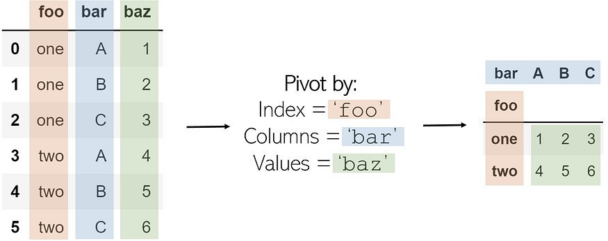
The code to pivot a DataFrame named df is as follows:

df.pivot(index='foo', columns='bar', values='baz')

To memorize: A pivot is — outside the realm of data manipulation — a turn around some sort of object. In sports, one can ‘pivot’ around their foot to spin: pivots in pandas are similar. The state of the original DataFrame is pivoted around central elements of a DataFrame into a new one. Some elements very literally pivot in that they are rotated or transformed (like column ‘bar’).

Melt

Melting can be thought of as an ‘unpivot,’ in that it converts matrix-based data (has two dimensions) into list-based data (columns represent values and rows indicate unique data points), whereas pivots do the opposite. Consider a two-dimensional matrix with one dimension ‘B’ and ‘C’ (column names), with the other dimension ‘a’, ‘b’, and ‘c’ (row indices).

We select an ID, one of the dimensions, and a column/columns to contain values. The column(s) that contain values are transformed into two columns: one for the variable (the name of the value column) and another for the value (the number contained in it).

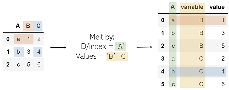
The result is every combination of the ID column’s values (a, b, c) and the value columns (B, C), with its corresponding value, organized in list format.

The melt operation can be performed like such on DataFrame df:

df.melt(id_vars=['A'], value_vars=['B','C'])

To memorize: Melting something like a candle is to turn a solidified and composite object into several much smaller, individual elements (wax droplets). Melting a two-dimensional DataFrame unpacks its solidified structure and records its pieces as individual entries in a list.

Explode

Exploding is a helpful method to get rid of lists in the data. When a column is exploded, all lists inside of it are listed as new rows under the same index (to prevent this, simply call .reset_index() afterward). Non-list items like strings or numbers are not affected, and empty lists are NaN values (you can cleanse these using .dropna()).

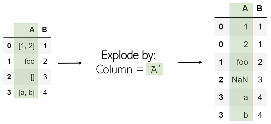
Exploding a column ‘A’ in DataFrame df is very simple:

df.explode(‘A’)

To remember: Exploding something releases all its internal contents — exploding a list separates its elements.

Stack

Stacking takes a DataFrame of any size and ‘stacks’ the columns as subindices of existing indices. Hence, the resulting DataFrame has only one column and two levels of indices.

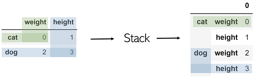
Stacking a table named df is as simple as df.stack().

In order to access the value of, say, the dog’s height, simply call an index-based retrieval twice, like df.loc[‘dog’].loc[‘height’].

To remember: Visually, stack takes the two-dimensionality of a table and stacks the columns into multi-level indices.

Unstack

Unstacking takes a multi-index DataFrame and unstacks it, converting the indices in a specified level into columns of a new DataFrame with its corresponding values. Calling a stack followed by an unstack on a table will not change it (excusing the existence of a ‘0’).

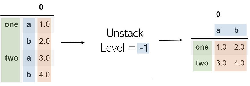
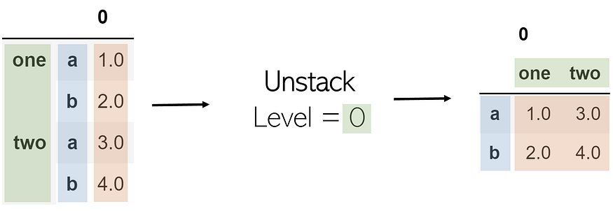
A parameter in unstacking is its level. In list indexing, an index of -1 will return the last element; this is the same with levels. A level of -1 indicates that the last index level (the one rightmost) will be unstacked. As a further example, when the level is set to 0 (the first index level), values in it become columns and the following index level (the second) becomes the transformed DataFrame’s index.

Unstacking can be performed the same as stacking, but with the level parameter: df.unstack(level=-1).

To remember: Unstack means “to undo a stack.”

Merge

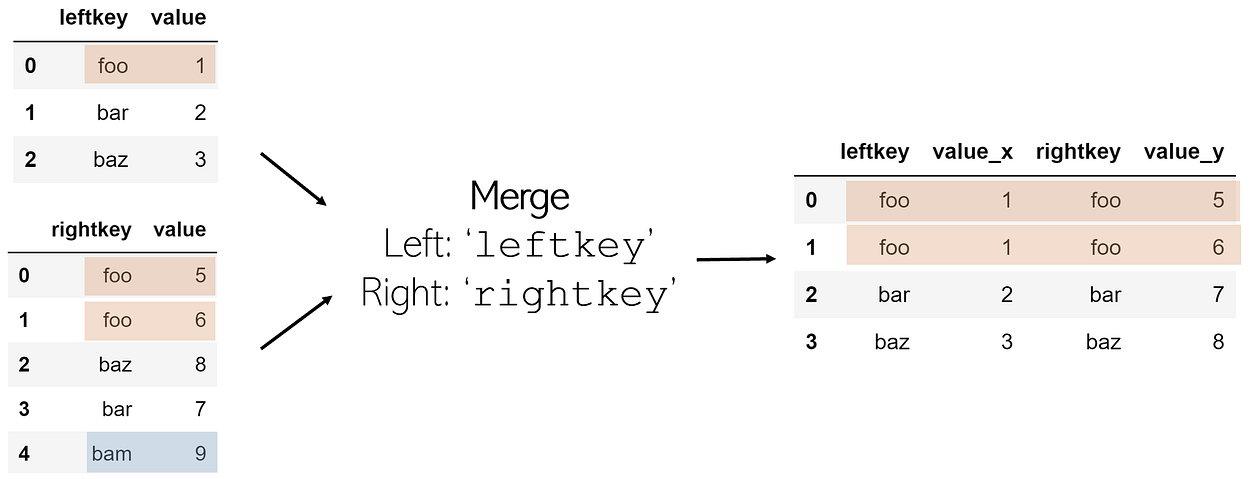
To merge two DataFrames is to combine them column-wise (horizontally) among a shared ‘key’. This key allows for the tables to be combined, even if they are not ordered similarly. The finished merged DataFrame will add suffixes _x and _y to value columns by default.

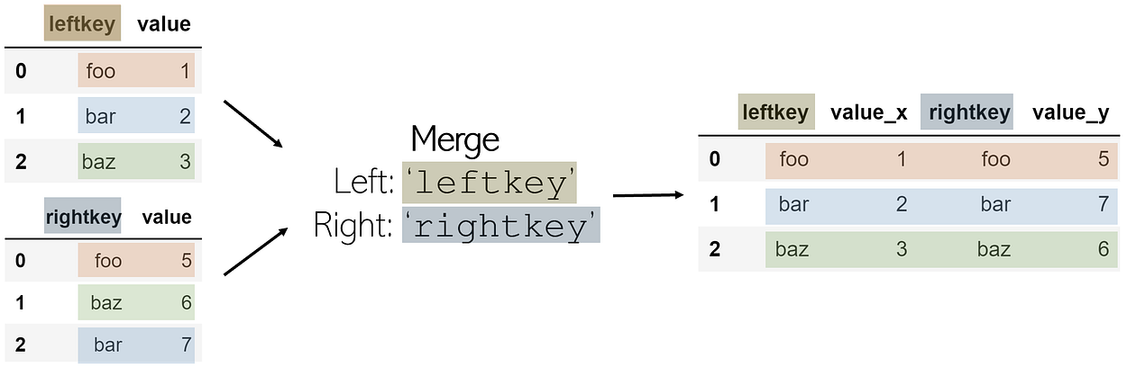
In order to merge two DataFrames df1 and df2 (where df1 contains the leftkey and df2 contains the rightkey), call:

df1.merge(df2, left_on='leftkey', right_on='rightkey')

Merges are not functions of pandas but are attached to a DataFrame. It is always assumed that the DataFrame in which the merge is being attached to is the ‘left table’, and the DataFrame called as a parameter in the function is the ‘right table’, with corresponding keys.

The merge function performs by default what is called an inner join: if each of the DataFrames has a key not listed in the other’s, it is not included in the merged DataFrame. On the other hand, if a key is listed twice in the same DataFrame, every combination of values for the same keys is listed in the merged table. For example, if df1 has 3 values for key foo and df2 had 2 values for the same key, there would be 6 entries with leftkey=foo and rightkey=foo in the final DataFrame.

To remember: You merge DataFrames like you merge lanes when driving — horizontally. Imagine each of the columns as one lane on the highway; in order to merge, they must combine horizontally.

Join

Joins are generally preferred over merge because it has a cleaner syntax and a wider range of possibilities in joining two DataFrames horizontally. The syntax of a join is as follows:

df1.join(other=df2, on='common_key', how='join_method')

When using joins, the common key column (analogous to right_on and left_on in merge) must be named the same name. The how parameter is a string referring to one of four methods join can combine two DataFrames:

• ‘left’: Include all elements of df1, accompanied with elements of df2 only if their key is a key of df1. Otherwise, the missing portion of the merged DataFrame for df2 will be marked as NaN.
• ‘right’: ‘left’, but on the other DataFrame. Include all elements of df2, accompanied with elements of df1 only if their key is a key of df2.
• ‘outer’: Include all elements from both DataFrames, even if a key is not present in the other’s — missing elements are marked as NaN.
• ‘inner’: Include only elements whose keys are present in both DataFrame keys (intersection). Default for merge.

To remember: If you’ve worked with SQL, the word ‘join’ should immediately be associated with column-wise addition. If not, ‘join’ and ‘merge’ have very similar meanings definition-wise.

Concat

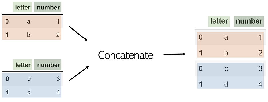
Whereas merges and joins work horizontally, concatenations, or concats for short, attach DataFrames row-wise (vertically). Consider, for example, two DataFrames df1 and df2 with the same column names, concatenated using pandas.concat([df1, df2]):

Although you can use concat for column-wise joining by turning the axis parameter to 1, it would be easier just to use join.

Note that concat is a pandas function and not one of a DataFrame. Hence, it takes in a list of DataFrames to be concatenated.

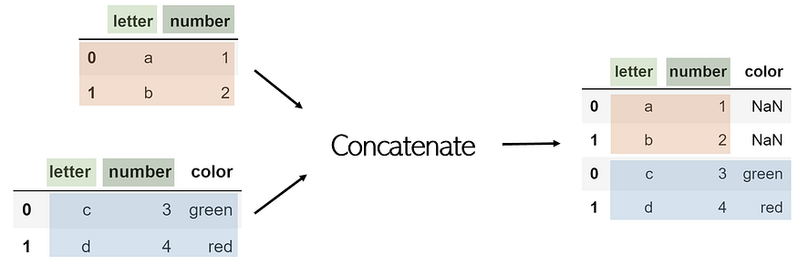
If a DataFrame has a column not included in the other, by default, it will be included, with missing values listed as NaN. To prevent this, add an additional parameter, join=’inner’, which will only concatenate columns both DataFrames have in common.

To remember: In lists and strings, additional items can be concatenated. Concatenation is the appendage of additional elements to an existing body, not the adding of new information (as is column-wise joining). Since each index/row is an individual item, concatenation adds additional items to a DataFrame, which can be thought of as a list of rows.

Append is another method to combine two DataFrames, but it performs the same functionality as concat and is less efficient and versatile.

Sometimes built-in functions aren’t enough.

Although these functions cover a wide range of what you may need to manipulate your data for, sometimes the data manipulation required is too complex for one or even a series of functions to perform. Explore complex data manipulation methods like parser functions, iterative projection, efficient parsing, and more here.

Original. Reposted with permission.

Related:

• Exploratory Data Analysis on Steroids
• How to Prepare Your Data
• Introduction to Pandas for Data Science