Simple Python Package for Comparing, Plotting & Evaluating Regression Models

By Ajay Arunachalam, Orebro University

I always believe in democratizing AI and machine learning, and spreading the knowledge in such a way, to cater the larger audiences in general, to harness the power of AI. An attempt inline to this is the development of the python package “regressormetricgraphplot” that is aimed to help users plot the evaluation metric graph with single line code for different widely used regression model metrics comparing them at a glance. With this utility package, it also significantly lowers the barrier for the practitioners to evaluate the different machine learning algorithms in an amateur fashion by applying it to their everyday predictive regression problems.

Before we dwell into the package details, let’s understand a few basic concepts in simple layman terms.

In general, the modeling pipeline involves the pre-processing stage, fitting the machine learning algorithms, and followed by their evaluation. In the figure below, as an example the modeling steps for ensemble learning is depicted. The block A includes the data processing like cleaning, wrangling, aggregation, deriving new features, feature selection, etc. The block B & C depicts the ensemble learning where the pre-processed data is input to the individual models in Layer-1 which are evaluated and tuned. The input to Layer-2 includes predictions from the previous Layer-1 where then the voting ensemble scheme is used to derive the final predictions. The results are combined using the average. Finally, the block D shows the model evaluation and result interpretation. The data is split (70:30 ratio) into training and testing data. The three standalone ML algorithms namely Linear Regression, Random Forest and XGBoost were used. All the models were created with tuned parameters, and then finally a Voting Regression model is used.

Modeling Pipeline Ensemble Learning Example

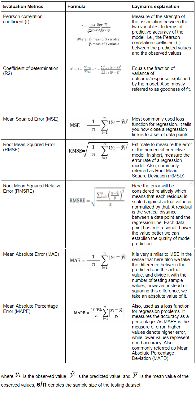
Different regression metrics were used for evaluation. Let’s discuss each of them with their formulae, and corresponding simple explanation.

A voting regressor is an ensemble meta-estimator that fits base regressors each on the whole dataset. It then averages the individual predictions to form a final prediction as shown below.

Getting Started

 
Terminal Installation

$ pip install regressormetricgraphplot

$ git clone https://github.com/ajayarunachalam/RegressorMetricGraphPlot
$ cd RegressorMetricGraphPlot
$ python setup.py install

 
Notebook

!git clone https://github.com/ajayarunachalam/RegressorMetricGraphPlot.git
cd RegressorMetricGraphPlot/

Just replace the line ‘from CompareModels import *’ with ‘from regressioncomparemetricplot import CompareModels’

Follow the rest as demonstrated in the demo example [here] — (https://github.com/ajayarunachalam/RegressorMetricGraphPlot/blob/main/regressormetricgraphplot/demo.ipynb)

 
Installation with Anaconda

If you installed your Python with Anaconda you can run the following commands to get started:

# Clone the repository
git clone https://github.com/ajayarunachalam/RegressorMetricGraphPlot.git
cd RegressorMetricGraphPlot

# Create new conda environment with Python 3.6
conda create — new your-env-name python=3.6

# Activate the environment
conda activate your-env-name

# Install conda dependencies
conda install — yes — file conda_requirements.txt

# Instal pip dependencies
pip install requirements.txt

CODE WALKTHROUGH

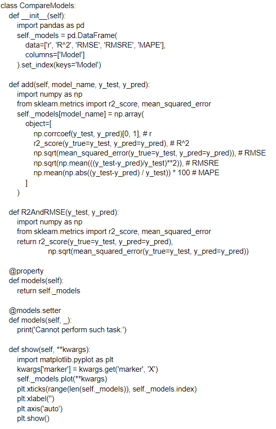
USAGE

plot = CompareModels()
plot.add(model_name=“Linear Regression”, y_test=y_test, y_pred=y_pred)
plot.show(figsize=(10, 5))

# Metrics
CompareModels.R2AndRMSE(y_test=y_test, y_pred=y_pred)

COMPLETE DEMO

 
Comprehensive demonstrations can be found in the Demo.ipynb file.

CONTACT

 
If there’s some metrics implementation you would like to add or add in some examples feel free to do so. You can reach me at ajay.arunachalam08@gmail.com

Always Keep Learning & Sharing Knowledge!!!

 
Bio: Ajay Arunachalam (personal website) is a Postdoctoral Researcher (Artificial Intelligence) at Centre for Applied Autonomous Sensor Systems, Orebro University, Sweden. Prior to this, he was working as a Data Scientist at True Corporation, a Communications Conglomerate, working with Petabytes of data, building & deploying deep models in production. He truly believes that Opacity in AI systems is need of the hour, before we fully accept the power of AI. With this in mind, he has always strived to democratize AI, and be more inclined towards building Interpretable Models. His interest is in Applied Artificial Intelligence, Machine Learning, Deep Learning, Deep RL, and Natural Language Processing, specifically learning good representations. From his experience working on real-world problems, he fully acknowledges that finding good representations is the key in designing the system that can solve interesting challenging real-world problems, that go beyond human-level intelligence, and ultimately explain complicated data for us that we don't understand. In order to achieve this, he envisions learning algorithms that can learn feature representations from both unlabelled and labelled data, be guided with and/or without human interaction, and that are on different levels of abstractions in order to bridge the gap between low-level data and high-level abstract concepts.

Original. Reposted with permission.

Related:

• Model Evaluation Metrics in Machine Learning
• PyCaret 2.1 is here: What’s new?
• Most Popular Distance Metrics Used in KNN and When to Use Them