The Inferential Statistics Data Scientists Should Know
The foundations of Data Science and machine learning algorithms are in mathematics and statistics. To be the best Data Scientists you can be, your skills in statistical understanding should be well-established. The more you appreciate statistics, the better you will understand how machine learning performs its apparent magic.

If you want to become a successful Data Scientist, you must know your basics. Mathematics and Statistics are the basic building blocks of Machine Learning algorithms. It is noteworthy to understand the techniques behind various Machine Learning algorithms to know how and when to use them. Now, what is Statistics?
Statistics is a mathematical science concerning Data collection, Analysis, Interpretation, and Presentation of data. It is one of the key fundamental skills needed for data science. Any specialist in data science would surely advise learning statistics.
In this article, I will discuss Inferential Statistics, which is one of the most prominent notions in statistics for data science.
Descriptive Statistics
Descriptive Statistics is a major branch of statistics that supports describing a huge amount of data with charts and tables. It neither permits us to draw inferences about the population nor reach an Inference regarding any of our hypotheses. Descriptive Statistics, by simply describing our collected dataset, enables us to present raw data in a more meaningful way.
Population and Sampling methods
The population contains all the data points from a set of data, while a sample consists of few observations selected from the population. The sample from the population should be selected such that it has all the properties that a population has. Population’s measurable properties such as mean, standard deviation, etc., are called parameters, while Sample’s measurable property is known as a statistic.
We create samples using any of the Sampling methods, which can be either probability-based and non-probability-based. In this blog, we’ll be focusing only on probability sampling techniques.
Probability Sampling: This is a sampling technique in which samples from a large population are collected using the theory of probability. There are three types of probability sampling:
- Random Sampling:In this method, each member of the population has an equal chance of being selected in the sample.
Systematic Sampling: In Systematic sampling, every nth record is chosen from the population to be a part of the sample.

Stratified Sampling: In Stratified sampling, a stratum is used to form samples from a large population. A stratum is a subset of the population that shares at least one common characteristic. After this, the random sampling method is used to select a sufficient number of subjects from each stratum.
Why do we need Inferential Statistics?
In contrast to Descriptive Statistics, rather than having access to the whole population, we often have a limited number of data.
In such cases, Inferential Statistics come into action. For example, we might be interested in finding the average of the entire school’s exam marks. It is not reasonable because we might find it impracticable to get the data we need. So, rather than getting the entire school’s exam marks, we measure a smaller sample of students (for example, a sample of 50 students). This sample of 50 students will now describe the complete population of all students of that school.
Simply put, Inferential Statistics make predictions about a population based on a sample of data taken from that population.
The technique of Inferential Statistics involves the following steps:
- First, take some samples and try to find one that represents the entire population accurately.
- Next, test the sample and use it to draw generalizations about the whole population.
There are two main objectives of inferential statistics:
- Estimating parameters: We take a statistic from the collected data, such as the standard deviation, and use it to define a more general parameter, such as the standard deviation of the complete population.
- Hypothesis testing: Very beneficial when we are looking to gather data on something that can only be given to a very confined population, such as a new drug. If we want to know whether this drug will work for all patients (“complete population”), we can use the data collected to predict this (often by calculating a z-score).
Statistical terminologies
Throughout the entire article, I will be using the below mentioned statistical terminology quite often:
- Statistic: A Single measure of some attribute of a sample. For e.g., the Mean/Median/Mode of a sample of Data Scientists in Bangalore.
- Population Statistic: The statistic of the entire population in context. For e.g., Population mean for the salary of the entire population of Data Scientists across India.
- Sample Statistic: The statistic of a group taken from a population. For e.g., the Mean salaries of all Data Scientists in New york.
- Standard Deviation: It is the amount of variation in the population data, given by σ.
- Standard Error: It is the amount of variation in the sample data. It is related to Standard Deviation as σ/√n, where n is the sample size.
Probability
The probability of an event refers to the likelihood that the event will occur.
Some important terms in probability:
- Random Experiment: Random experiment or statistical experiment is an experiment in which all the possible outcomes of the experiments are already known. The experiment can be repeated numerous times under identical or similar conditions.
- Sample space: The sample space of a random experiment is the collection or set of all the possible outcomes of a random experiment.
- Event: A subset of sample space is called an event.
- Trial: Trial refers to a special type of experiment in which we have two types of possible outcomes: success or failure with varying Success probability.
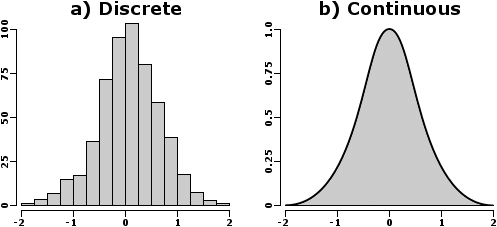
- Random Variable: A variable whose value is subject to variations due to randomness is called a random variable. A random variable is of two types: Discrete and Continuous variables. Mathematically, we can say that a real-valued function X: S -> R is called a random variable where S is probability space and R is a set of real numbers.
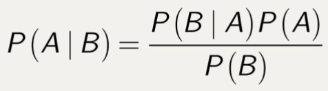
Conditional Probability
Conditional probability is the probability of a particular event A, given a certain condition which has already occurred, i.e., B. Then conditional probability, P(A|B) is defined as,
Probability Distribution and Distribution function
The mathematical function describing the randomness of a random variable is called a probability distribution. It is a depiction of all possible outcomes of a random variable and its associated probabilities.
Sampling Distribution
The probability distribution of statistics of a large number of samples selected from the population is called a sampling distribution. When we increase the size of the sample, the sample mean becomes more normally distributed around the population mean. The variability of the sample decreases as we increase the sample size.
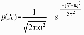
Normal distribution
The normal distribution is a continuous probability distribution that is described by Normal Equation,
A Normal distribution curve is symmetrical on both sides of the mean, so the right side of the center is a mirror image of the left side.
The area under the normal distribution curve represents probability, and the total area under the curve sums to one.
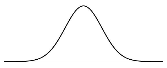
A Normal distribution curve has the following properties:
- mean, median, and mode are equal.
- The curve is symmetric, with half of the values on the left and half of the values on the right.
- The area under the curve is 1.
A Normal distribution follows the Empirical rule, which states that:
- 68%of the data falls within 1 standard deviation of the mean
- 95%of the data falls within 2 standard deviations of the mean
- 7%of the data falls within 3 standard deviations of the mean.
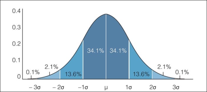
Empirical rule. Image credit.
The normal distribution is the most significant probability distribution in statistics because many continuous data in nature and psychology displays this bell-shaped curve when compiled and graphed.
For example, if we randomly sampled 50 people, we would expect to see a normal distribution frequency curve for many continuous variables, such as IQ, height, weight, and blood pressure.
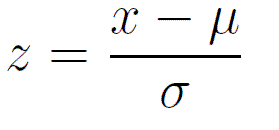
Z statistic
For calculating the probability of occurrence of an event, we need the z statistic. The formula for calculating the z statistic is

where x is the value for which we want to calculate the z value. μ and σ are the population mean and standard deviation, respectively.
Basically, what we are doing here is standardizing the normal curve by moving the mean to 0 and converting the standard deviation to 1. The z statistic is essentially the distance of the value from the mean calculated in standard deviation terms. So a z statistic of 1.67 means that the value is 1.67 standard deviations away from the mean in the positive direction. We then find the probability by looking up the corresponding z statistic from the z table.
Central Limit Theorem
It states that when plotting a sampling distribution of means, the mean of sample means will be equal to the population mean. And the sampling distribution will approach a normal distribution with variance equal to σ/√n where σ is the standard deviation of population and n is the sample size.
Some points to note here:
- Central Limit Theorem holds irrespective of the shape and type of distribution of the population, be it bi-modal, right-skewed, etc. The shape of the Sampling Distribution will remain the same (bell-shaped). This gives us a mathematical advantage to estimate the population statistic no matter the shape of the population.
- The number of samples has to be sufficient (generally more than 50) to convincingly produce a normal curve distribution. Also, caution has to be taken to keep the sample size fixed since any change in sample size will change the shape of the sampling distribution, and it will no longer be bell-shaped.
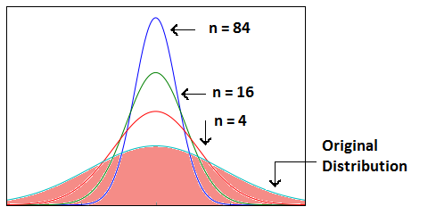
- The greater the sample size, the lower the standard error and the greater the accuracy in determining the population mean from the sample mean. As we increase the sample size, the sampling distribution squeezes from both sides, giving us a better estimate of the population statistic since it lies somewhere in the middle of the sampling distribution (usually). The below image will help you visualize the effect of sample size on the shape of the distribution.
Now, since we have collected the samples and plotted their means, it is important to know where the population mean lies for a particular sample mean and how confident can we be about it, which is calculated using Confidence Interval.
Confidence Interval
Confidence Interval is used to express the precision and uncertainty associated with a particular sampling method. A confidence interval consists of three parts.
- A confidence level.
- A statistic.
- A margin of error.
The confidence level describes the uncertainty of a sampling method (it's the probability part of the confidence interval). The statistic and the margin of error define an interval estimate that describes the precision of the method. The interval estimate of a confidence interval is defined by the sample statistic + margin of error.
The margin of error is found by multiplying the standard error of the mean and the z-score.
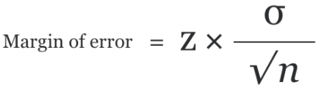
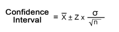
And the Confidence interval is defined as:
Margin of Error. Image credit.
A confidence interval having a value of 90% indicates that we are 90% sure that the actual mean is within our confidence interval.
Hypothesis Testing
Hypothesis testing is a part of statistics in which we make assumptions about the population parameter. So, hypothesis testing mentions a proper procedure by analyzing a random sample of the population to accept or reject the assumption.
Hypothesis testing is the way of trying to make sense of assumptions by looking at the sample data.
Type of Hypothesis
The best way to determine whether a statistical hypothesis is true would be to examine the entire population. Since that is often impractical, researchers typically examine a random sample from the population. If sample data are not consistent with the statistical hypothesis, the hypothesis is rejected.
There are two types of statistical hypotheses.
- Null hypothesis. The null hypothesis, denoted by Ho, is usually the hypothesis that sample observations result purely from chance.
- Alternative hypothesis. The alternative hypothesis, denoted by H1 or Ha, is the hypothesis that sample observations are influenced by some non-random cause.
Steps of Hypothesis Testing
The process to determine whether to reject a null hypothesis or to fail to reject the null hypothesis, based on sample data. This process, called hypothesis testing, consists of four steps.
- State the hypotheses. This involves stating the null and alternative hypotheses, and both should be mutually exclusive. That is, if one is true, the other must be false.
- Formulate an analysis plan. It describes how to use sample data to evaluate the null hypothesis. This evaluation often focuses on a single test statistic. Here we choose the significance level (α) among 0.01, 0.05, or 0.10 and also determine the test method.
- Analyze sample data. Find the value of the test statistic (mean score, proportion, t statistic, z-score, etc.) and p-value described in the analysis plan.
- Interpret results. Apply the decision rule described in the analysis plan. If the value of the test statistic is unlikely, based on the null hypothesis, reject the null hypothesis.
Errors in hypothesis testing
We have explained what is hypothesis testing and the steps to do the testing. Now, while performing the hypothesis testing, there might be some errors.
- Type I error. A Type I error occurs when the researcher rejects a null hypothesis when it is true. The probability of committing a Type I error is called the significance level. This probability is also called alpha and is often denoted by α.
- Type II error. A Type II error occurs when the researcher fails to reject a false null hypothesis. The probability of committing a Type II error is called beta and is often denoted by β. The probability of not committing a Type II error is called the Power of the test.
Terms in Hypothesis testing
Significance level
The significance level is defined as the probability of the case when we reject the null hypothesis, but in actuality, it is true. For example, a 0.05 significance level indicates that there is a 5% risk in assuming that there is some difference when, in actuality, there is no difference. It is denoted by alpha (α).
The above figure shows that the two shaded regions are equidistant from the null hypothesis, each having a probability of 0.025 and a total of 0.05, which is our significance level. The shaded region in case of a two-tailed test is called the critical region.
P-value
The p-value is defined as the probability of seeing a t-statistic as extreme as the calculated value if the null hypothesis value is true. A low enough p-value is the ground for rejecting the null hypothesis. We reject the null hypothesis if the p-value is less than the significance level.
Z-test
A Z-test is mainly used when the data is normally distributed. We find the Z-statistic of the sample means and calculate the z-score. Z-score is given by the formula,
Z-score.
Z-test is mainly used when the population mean and standard deviation are given.
T-test
T-tests are very much similar to the z-scores, the only difference being that instead of the Population Standard Deviation, we now use the Sample Standard Deviation. The rest is the same as before, calculating probabilities on the basis of t-values.
The Sample Standard Deviation is given as:
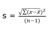
where n-1 is Bessel’s correction for estimating the population parameter.
Another difference between z-scores and t-values is that t-values are dependent on the Degree of Freedom of a sample. Let us define what degree of freedom is for a sample.
The Degree of Freedom — It is the number of variables that have the choice of having more than one arbitrary value. For example, in a sample of size 10 with a mean of 10, 9 values can be arbitrary, but the 10th value is forced by the sample mean.
Points to note about the t-tests:
- The greater the difference between the sample mean and the population mean, the greater the chance of rejecting the Null Hypothesis.
- Greater the sample size, the greater the chance of rejection of the Null Hypothesis.
Different types of T-test
One Sample T-test
The one-sample t-test compares the mean of sample data to a known value. So, if we have to compare the mean of sample data to the population mean, we use the One-Sample T-test.
We can run a one-sample T-test when we do not have the population S.D., or we have a sample of size less than 30.
t-statistic is given by:

where, X(bar) is the sample mean, μ the population mean, s the sample standard deviation, and N the sample size.
Two sample T-test
We use a two-sample T-test when we want to evaluate whether the mean of the two samples is different or not. In a two-sample T-test, we have another two categories:
- Independent Sample T-test: Independent sample means that the two different samples should be selected from two completely different populations. In other words, we can say that one population should not be dependent on the other population.

- Paired T-test: If our samples are connected in some way, we have to use the paired t-test. Here, ‘connecting’ means that the samples are connected as we are collecting data from the same group two times, e.g., blood tests of patients of a hospital before and after medication.

Chi-square test
The Chi-square test is used in the case when we have to compare categorical data.
The Chi-square test is of two types. Both use chi-square statistics and distribution for different purposes.
- The goodness of fit: It determines if sample data of categorical variables match with population or not.
- Test of Independence: It compares two categorical variables to find whether they are related to each other or not.
Chi-square statistic is given by:

ANOVA (Analysis of variance)
ANOVA (Analysis of Variance) is used to check if at least one of two or more groups have statistically different means. Now, the question arises — Why do we need another test for checking the difference of means between independent groups? Why can we not use multiple t-tests to check for the difference in means?
The answer is simple. Multiple t-tests will have a compound effect on the error rate of the result. Performing a t-test thrice will give an error rate of ~15%, which is too high, whereas ANOVA keeps it at 5% for a 95% confidence interval.
To perform an ANOVA, you must have a continuous response variable and at least one categorical factor with two or more levels. ANOVA requires data from approximately normally distributed populations with equal variances between factor levels.
There are two types of ANOVA test:
- One-way ANOVA: when only 1 independent variable is considered.
- Two-way ANOVA: when 2 independent variables are considered.
- N-way ANOVA: when N number of independent variables are considered.
Correlation Coefficient (R or r)
It is used to measure the strength between two variables. It is simply the square root of the coefficient of Determination and ranges from -1 to 1 where 0 represents no correlation, and 1 represents positive strong correlation while -1 represents negative strong correlation.
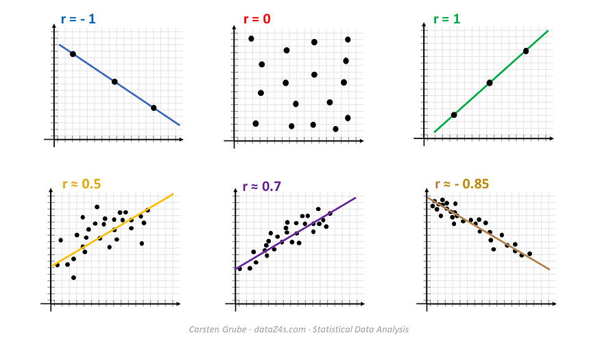
Scatter plot showing the coefficient of correlation. Image credit.
References
https://stattrek.com/tutorials/ap-statistics-tutorial.aspx
https://www.mygreatlearning.com/blog/inferential-statistics-an-overview/
https://en.wikipedia.org/wiki/Statistical_inference
https://deepai.org/machine-learning-glossary-and-terms/inferential-statistics
https://www.edureka.co/blog/statistics-and-probability/
Related: