An introduction to Explainable AI (XAI) and Explainable Boosting Machines (EBM)
Understanding why your AI-based models make the decisions they do is crucial for deploying practical solutions in the real-world. Here, we review some techniques in the field of Explainable AI (XAI), why explainability is important, example models of explainable AI using LIME and SHAP, and demonstrate how Explainable Boosting Machines (EBMs) can make explainability even easier.
By Chaitanya Krishna Kasaraneni, Data Science Intern at Predmatic AI.

Photo by Rock’n Roll Monkey on Unsplash.
In recent times, machine learning has become the core of developments in many fields such as sports, medicine, science, and technology. Machines (computers) have become so intelligent that they even defeated professionals in games like Go. Such developments raise questions if machines would also make for better drivers (autonomous vehicles) or even better doctors.
In many machine learning applications, the users rely on the model to make decisions. But, a doctor certainly cannot operate on a patient simply because “the model said so.” Even in low-risk situations, such as when choosing a movie to watch from a streaming platform, a certain measure of trust is required before we surrender hours of our time based on a model.
Despite the fact that many machine learning models are black boxes, understanding the rationale behind the model’s predictions would certainly help users decide when to trust or not to trust their predictions. This “understanding the rationale” leads to the concept called Explainable AI (XAI).
What is Explainable AI (XAI)?
Explainable AI refers to methods and techniques in the application of artificial intelligence technology (AI) such that the results of the solution can be understood by human experts. [Wikipedia]
How is Explainable AI different from Artificial Intelligence?


Difference Between AI and XAI.
In general, AI arrives at a result using an ML algorithm, but the architects of the AI systems do not fully understand how the algorithm reached that result.
On the other hand, XAI is a set of processes and methods that allows users to understand and trust the results/output created by a machine learning model/algorithm. XAI is used to describe an AI model, its expected impact, and potential biases. It helps characterize model accuracy, fairness, transparency, and outcomes in AI-powered decision-making. Explainable AI is crucial for an organization in building trust and confidence when putting AI models into production. AI explainability also helps an organization adopt a responsible approach to AI development.
Famous examples of such explainers are Local Interpretable Model-agnostic Explanations (LIME) and SHapley Additive exPlanations (SHAP).
- LIME explains the predictions of any classifier in an interpretable and faithful manner by learning an interpretable model locally around the prediction.
- SHAP is a game theoretic approach to explain the output of any machine learning model.
Explaining Predictions using SHAP
SHAP is a novel approach to XAI developed by Scott Lundberg here at Microsoft and eventually opened sourced.
SHAP has a strong mathematical foundation. It connects optimal credit allocation with local explanations using the classic Shapley values from game theory and their related extensions (see papers for details).
Shapley values
With Shapley values, each prediction can be broken down into individual contributions for every feature.
For example, consider your input data has 4 features (x1, x2, x3, x4) and the output of a model is 75, using Shapley values, you can say that feature x1 contributed 30, feature x2 contributed 20, feature x3 contributed -15, and feature x4 contributed 40. The sum of these 4 Shapley values is 30+20–15+40=75, i.e., the output of your model. This feels great, but sadly, these values are extremely hard to calculate.
For a general model, the time taken to compute Shapley values is exponential to the number of features. If your data has 10 features, this might still be okay. But if the data has more features, say 20, depending on your hardware, it might be impossible already. To be fair, if your model consists of trees, there are faster approximations to compute Shapley values, but it can still be slow.
SHAP using Python
In this article, we’ll be using red wine quality data to understand SHAP. The target value of this dataset is the quality rating from low to high (0–10). The input variables are the content of each wine sample, including fixed acidity, volatile acidity, citric acid, residual sugar, chlorides, free sulfur dioxide, total sulfur dioxide, density, pH, sulfates, and alcohol. There are 1,599 wine samples. The code can be found via this GitHub link.
In this post, we will build a random forest regression model and will use the TreeExplainer in SHAP. There is a SHAP Explainer for any ML algorithm — either tree-based or non-tree-based algorithms. It is called the KernelExplainer. If your model is a tree-based machine learning model, you should use the tree explainer TreeExplainer() that has been optimized to render fast results. If your model is a deep learning model, use the deep learning explainer DeepExplainer(). For all other types of algorithms (such as KNNs), use KernelExplainer().
The SHAP value works for either the case of a continuous or binary target variable.
Variable Importance Plot — Global Interpretability
A variable importance plot lists the most significant variables in descending order. The top variables contribute more to the model than the bottom ones and thus have high predictive power. Please refer to this notebook for code.
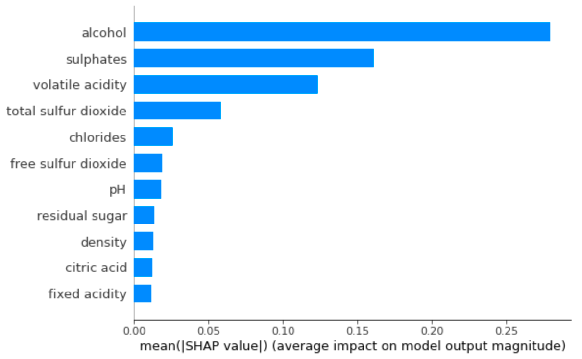
Variable Importance Plot using SHAP.
Summary Plot
Although the SHAP does not have built-in functions, you can output the plot using the matplotlib library.
The SHAP value plot can further show the positive and negative relationships of the predictors with the target variable.

Summary Plot.
This plot is made of all the dots in the train data. It demonstrates the following information:
- Variables are ranked in descending order.
- The horizontal location shows whether the effect of that value is associated with a higher or lower prediction.
- The color shows whether that variable is high (in red) or low (in blue) for that observation.
Using SHAP, we can generate partial dependence plots. The partial dependence plot shows the marginal effect one or two features have on the predicted outcome of a machine learning model (J. H. Friedman 2001). It tells whether the relationship between the target and a feature is linear, monotonic, or more complex.
Black-box explanations are much better than no explanation at all. However, as we have seen, both LIME and SHAP have some shortcomings. It would be better if the model is performing well and is interpretable at the same time—Explainable Boosting Machine (EBM) is a representative of such a method.
Explainable Boosting Machine (EBM)
EBM is a glassbox model designed to have accuracy comparable to state-of-the-art machine learning methods like Random Forest and BoostedTrees, while being highly intelligible and explainable.
The EBM Algorithm is a fast implementation of the GA²M algorithm. In turn, the GA²M algorithm is an extension of the GAM algorithm. Therefore, let’s start with what the GAM algorithm is.
GAM Algorithm
GAM stands for Generalized Additive Model. It is more flexible than logistic regression but still interpretable. The hypothesis function for GAM is as follows:

The key part to notice is that instead of a linear term ????ixi for a feature, now we have a function fi(xi). We will come back later to how this function is computed in EBM.
One limitation of GAM is that each feature function is learned independently. This prevents the model from capturing interactions between features and pushes the accuracy down.
GA²M algorithm
GA²M seeks to improve this. To do so, it also considers some pairwise interaction terms in addition to the function learned for each feature. This is not an easy problem to solve because there are a larger number of interaction pairs to consider, which increases compute time drastically. In GA²M, they use the FAST algorithm to pick up useful interactions efficiently. This is the hypothesis function for GA²M. Note the extra pairwise interaction terms.
By adding pairwise interaction terms, we get a stronger model while still being interpretable. This is because one can use a heatmap and visualize two features in 2D and their effect on the output clearly.
EBM Algorithm
Finally, let us talk about the EBM algorithm. In EBM, we learn each feature function fi(xi) using methods such as bagging and gradient boosting. To make the learning independent of the order of features, the authors use a very low learning rate and cycle through the features in a round robin fashion. The feature function fi for each feature represents how much each feature contributes to the model’s prediction for the problem and is hence directly interpretable. One can plot the individual function for each feature to visualize how it affects the prediction. The pairwise interaction terms can also be visualized on a heatmap as described earlier.
This implementation of EBM is also parallelizable, which is invaluable in large-scale systems. It also has the added advantage of having an extremely fast inference time.
Training the EBM
The EBM training part uses a combination of boosted trees and bagging. A good definition would probably be bagged boosted bagged shallow trees.
Shallow trees are trained in a boosted way. These are tiny trees (with a maximum of 3 leaves by default). Also, the boosting process is specific: Each tree is trained on only one feature. During each boosting round, trees are trained for each feature one after another. It ensures that:
- The model is additive.
- Each shape function uses only one feature.
This is the base of the algorithm, but other techniques further improve the performance:
- Bagging, on top of this base model.
- Optional bagging, for each boosting step. This step is disabled by default because it increases the training time.
- Pairwise interactions.
Depending on the task, the third technique can dramatically boost performance. Once a model is trained with individual features, a second pass is done (using the same training procedure) but with pairs of features. The pair selection uses a dedicated algorithm that avoids trying all possible combinations (which would be infeasible when there are many features).
Finally, after all these steps, we have a tree ensemble. These trees are discretized simply by running them with all the possible values of the input features. This is easy since all features are discretized. So the maximum number of values to predict is the number of bins for each feature. In the end, these thousands of trees are simplified to binning and scoring vectors for each feature.
EBM using Python
We will use the same red wine quality data to understand InterpretML. The code can be found via this GitHub Link.
Exploring Data
The “summary” of training data displays a histogram of the target variable.
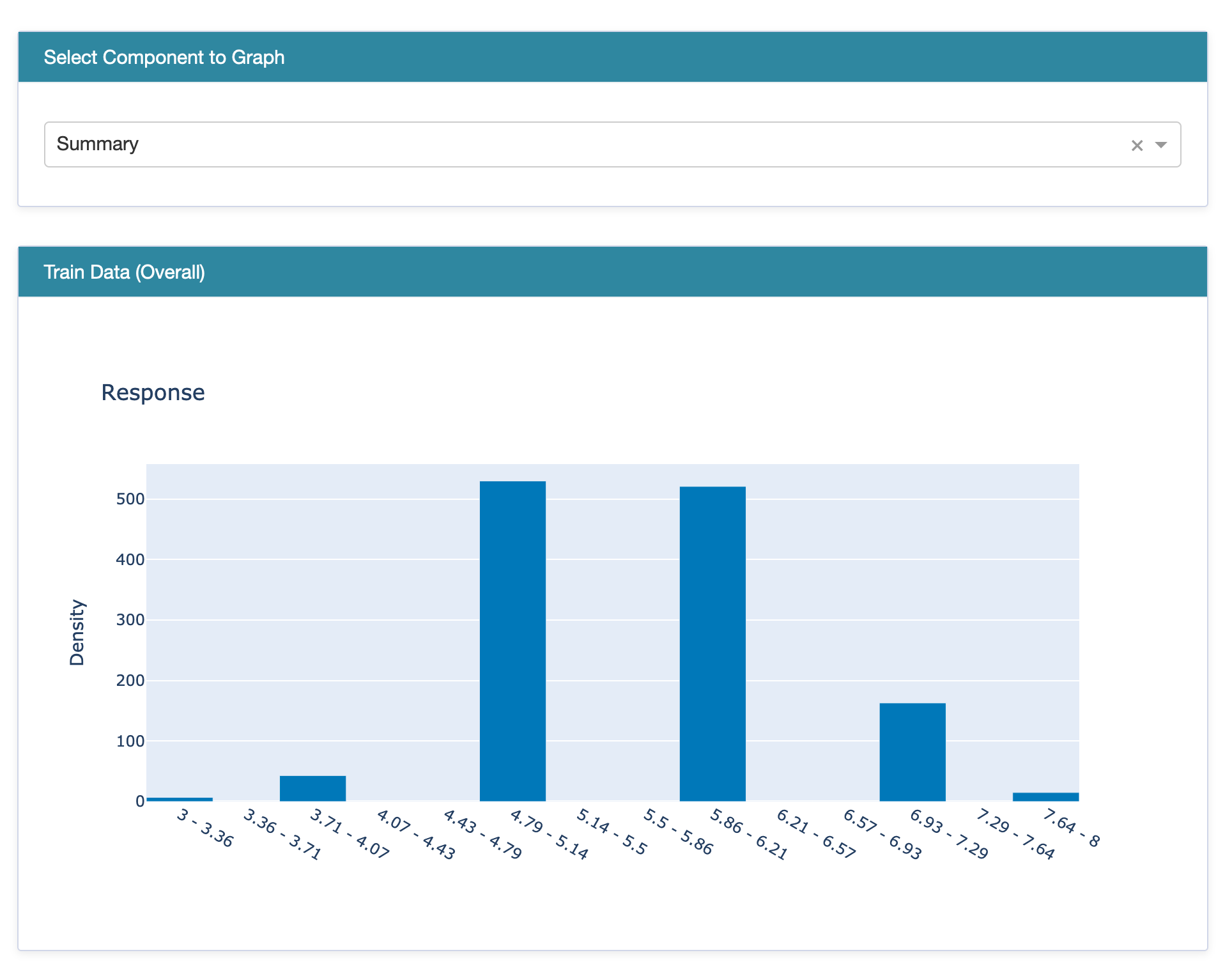
Summary displaying a histogram of Target.
When an individual feature (here fixed acidity) is selected, the graph shows the Pearson Correlation of that feature with the target. Also, a histogram of the selected feature is shown in blue color against the histogram of the target variable in red color.
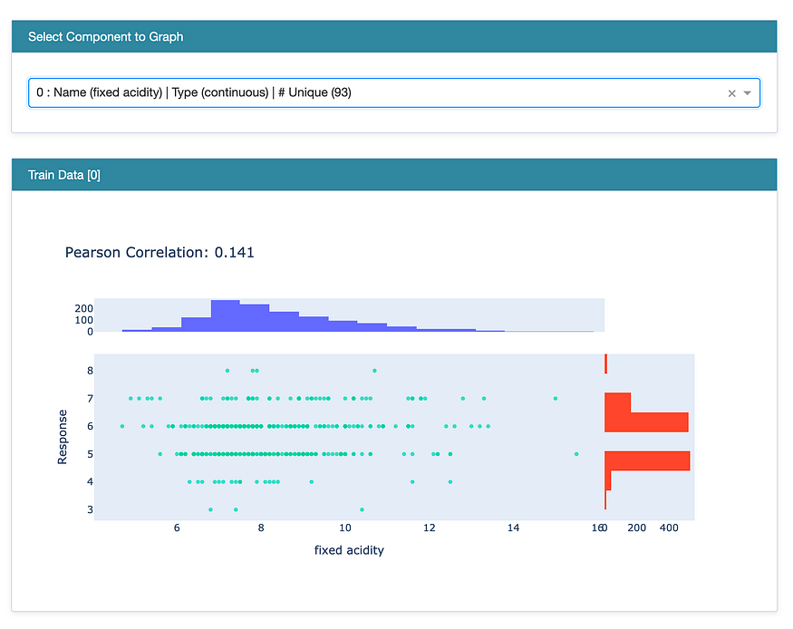
Individual Feature against Target.
Training the Explainable Boosting Machine (EBM)
The ExplainableBoostingRegressor() model of the InterpretML library with the default hyper-parameters is used here. RegressionTree() and LinearRegression() are also trained for comparison.
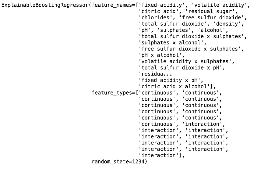
ExplainableBoostingRegressor Model.
Explaining EBM Performance
RegressionPerf() is used to assess the performance of each model on the test data. The R-squared value of EBM is 0.37, which outperforms the R-squared error of linear regression and regression tree models.
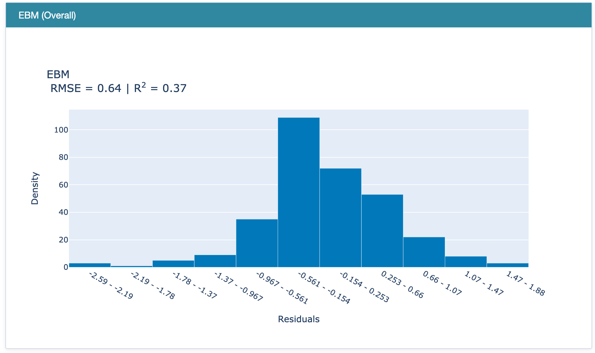
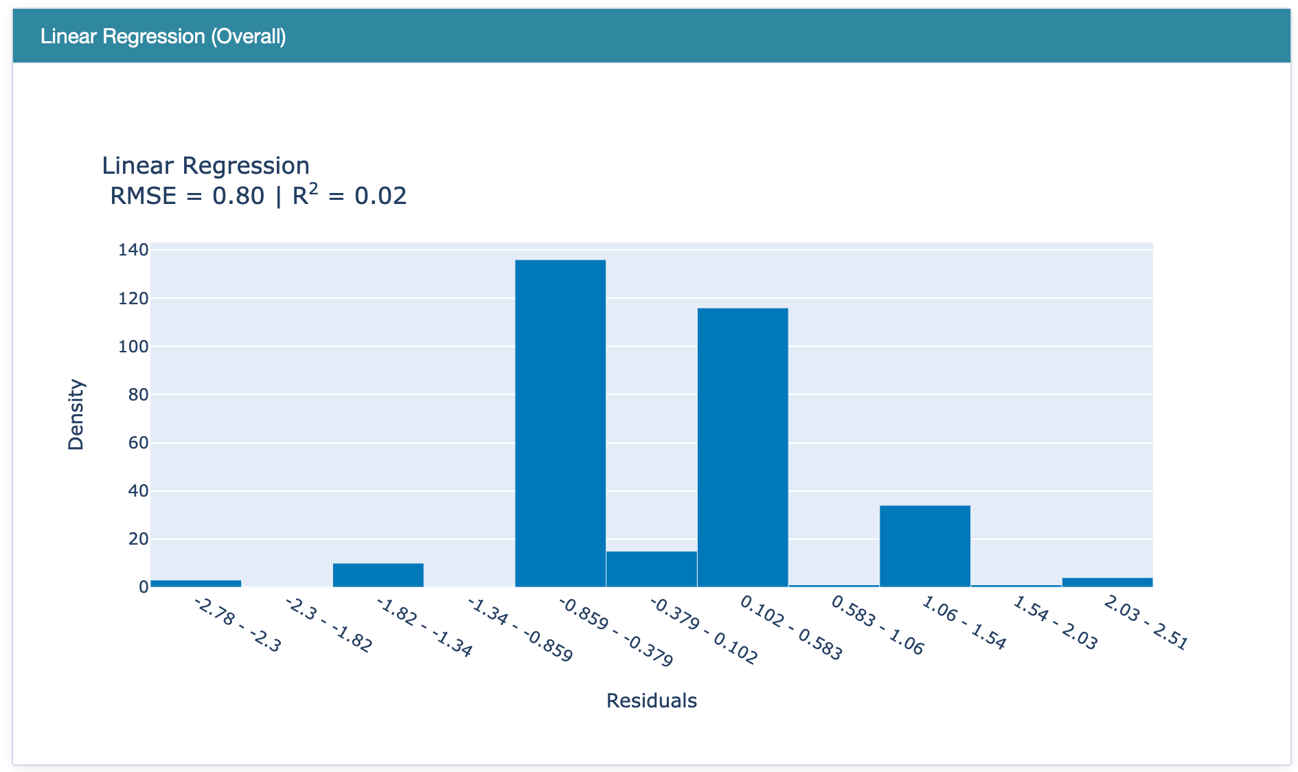
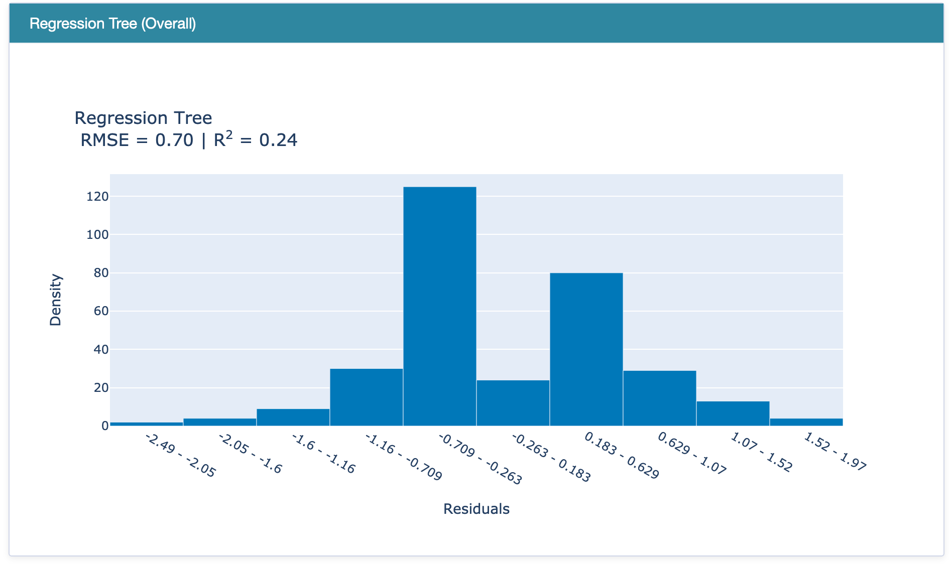
Performance of (a) EBM, (b) Linear Regression, and (c) Regression Tree.
The global and local interpretability of each model can also be generated using the model.explain_global() and model.explain_local()methods, respectively.
InterpretML also provides a feature to combine everything and generate an interactive dashboard. Please refer to the notebook for graphs and a dashboard.
Conclusion
With the increasing growth of requirements for explainability and existing shortcomings of the XAI models, the times when one had to choose between accuracy and explainability are long gone. EBMs can be as efficient as boosted trees while being as easily explainable as logistic regression.
Original. Reposted with permission.
Related: