Hands-On Reinforcement Learning Course, Part 2
Continue your learning journey in Reinforcement Learning with this second of two part tutorial that covers the foundations of the technique with examples and Python code.
By Pau Labarta Bajo, mathematician and data scientist.

Venice’s taxis by Helena Jankovičová Kováčová from Pexels.
This is part 2 of my hands-on course on reinforcement learning, which takes you from zero to HERO. Today we will learn about Q-learning, a classic RL algorithm born in the 90s.
If you missed part 1, please read it to get the reinforcement learning jargon and basics in place.
Today we are solving our first learning problem…
We are going to train an agent to drive a taxi!
Well, a simplified version of a taxi environment, but a taxi at the end of the day.
We will use Q-learning, one of the earliest and most used RL algorithms.
And, of course, Python.
All the code for this lesson is in this Github repo. Git clone it to follow along with today’s problem.

1. The taxi driving problem
We will teach an agent to drive a taxi using Reinforcement Learning.
Driving a taxi in the real world is a very complex task to start with. Because of this, we will work in a simplified environment that captures the 3 essential things a good taxi driver does, which are:
- pick up passengers and drop them at their desired destination.
- drive safely, meaning no crashes.
- drive them in the shortest time possible.
We will use an environment from OpenAI Gym, called the Taxi-v3 environment.
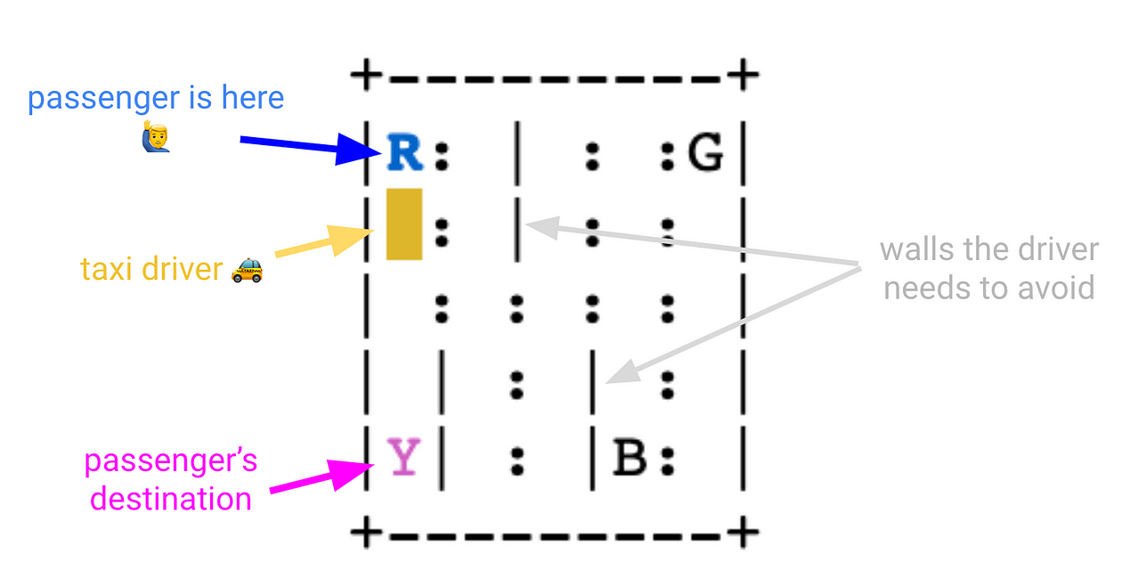
There are four designated locations in the grid world indicated by R(ed), G(reen), Y(ellow), and B(lue).
When the episode starts, the taxi starts off at a random square, and the passenger is at a random location (R, G, Y, or B).
The taxi drives to the passenger’s location, picks up the passenger, drives to the passenger’s destination (another one of the four specified locations), and then drops off the passenger. While doing so, our taxi driver needs to drive carefully to avoid hitting any wall, marked as |. Once the passenger is dropped off, the episode ends.
This is how the q-learning agent we will build drives today:
Before we get there, let’s understand well what are the actions, states, and rewards for this environment.
2. Environment, actions, states, rewards
notebooks/00_environment.ipynb
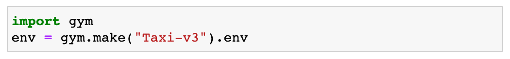
Let’s first load the environment:
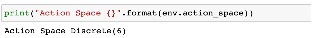
What are the actions the agent can choose from at each step?
- 0 drive down
- 1 drive up
- 2 drive right
- 3 drive left
- 4 pick up a passenger
- 5 drop off a passenger
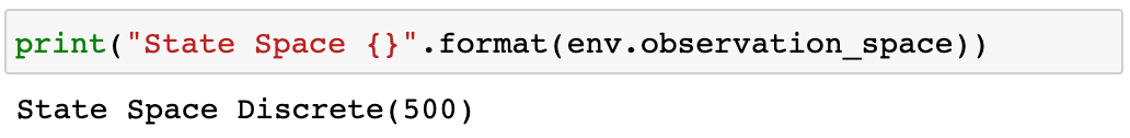
And the states?
- 25 possible taxi positions because the world is a 5×5 grid.
- 5 possible locations of the passenger, which are R, G, Y, B, plus the case when the passenger is in the taxi.
- 4 destination locations
which gives us 25 x 5 x 4 = 500 states.
What about rewards?
- -1 default per-step reward.
Why -1, and not simply 0? Because we want to encourage the agent to spend the shortest time, by penalizing each extra step. This is what you expect from a taxi driver, don’t you? - +20 reward for delivering the passenger to the correct destination.
- -10 reward for executing a pickup or dropoff at the wrong location.
You can read the rewards and the environment transitions (state, action ) → next_state from env.P.
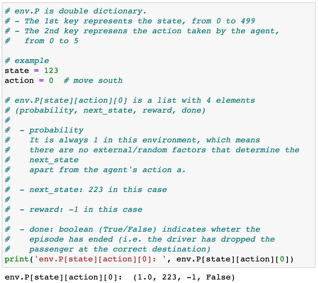
By the way, you can render the environment under each state to double-check this env.P vectors make sense:
From state=123:
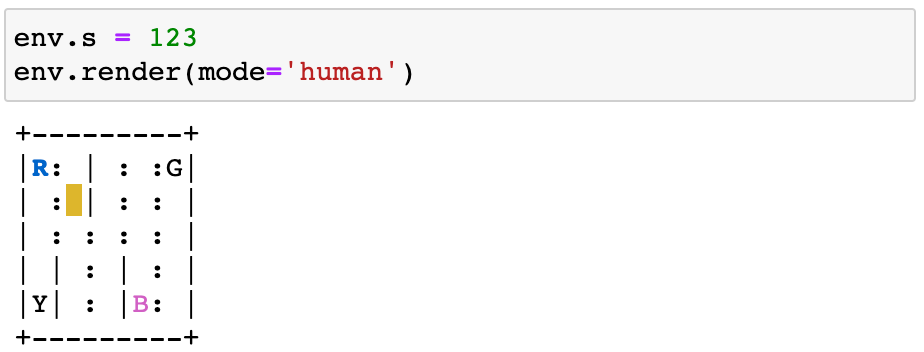
the agent moves south action=0 to get to state=223:
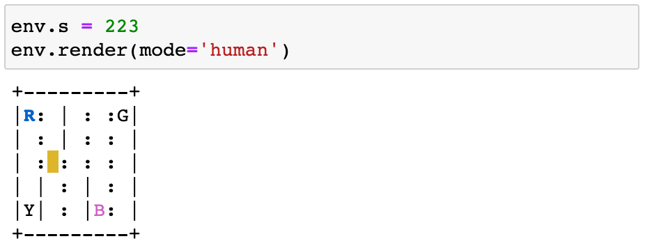
And the reward is -1, as neither the episode ended nor the driver incorrectly picked or dropped.
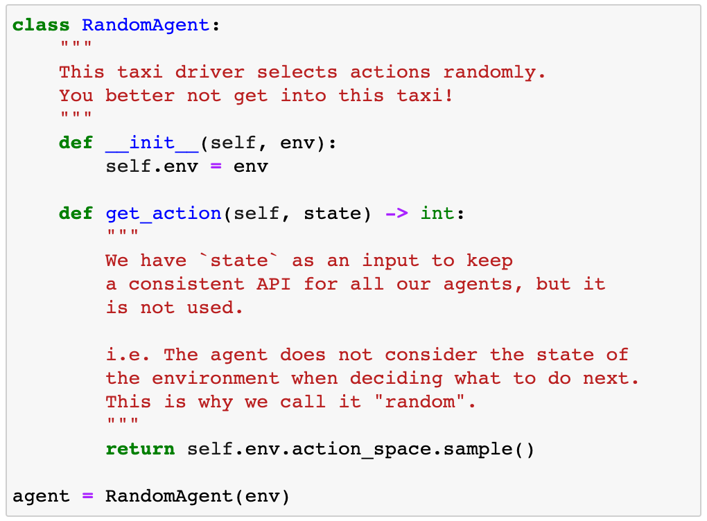
3. Random agent baseline
notebooks/01_random_agent_baseline.ipynb
Before you start implementing any complex algorithm, you should always build a baseline model.
This advice applies not only to Reinforcement Learning problems but Machine Learning problems in general.
It is very tempting to jump straight into the complex/fancy algorithms, but unless you are really experienced, you will fail terribly.
Let’s use a random agent as a baseline model.
We can see how this agent performs for a given initial state=198:
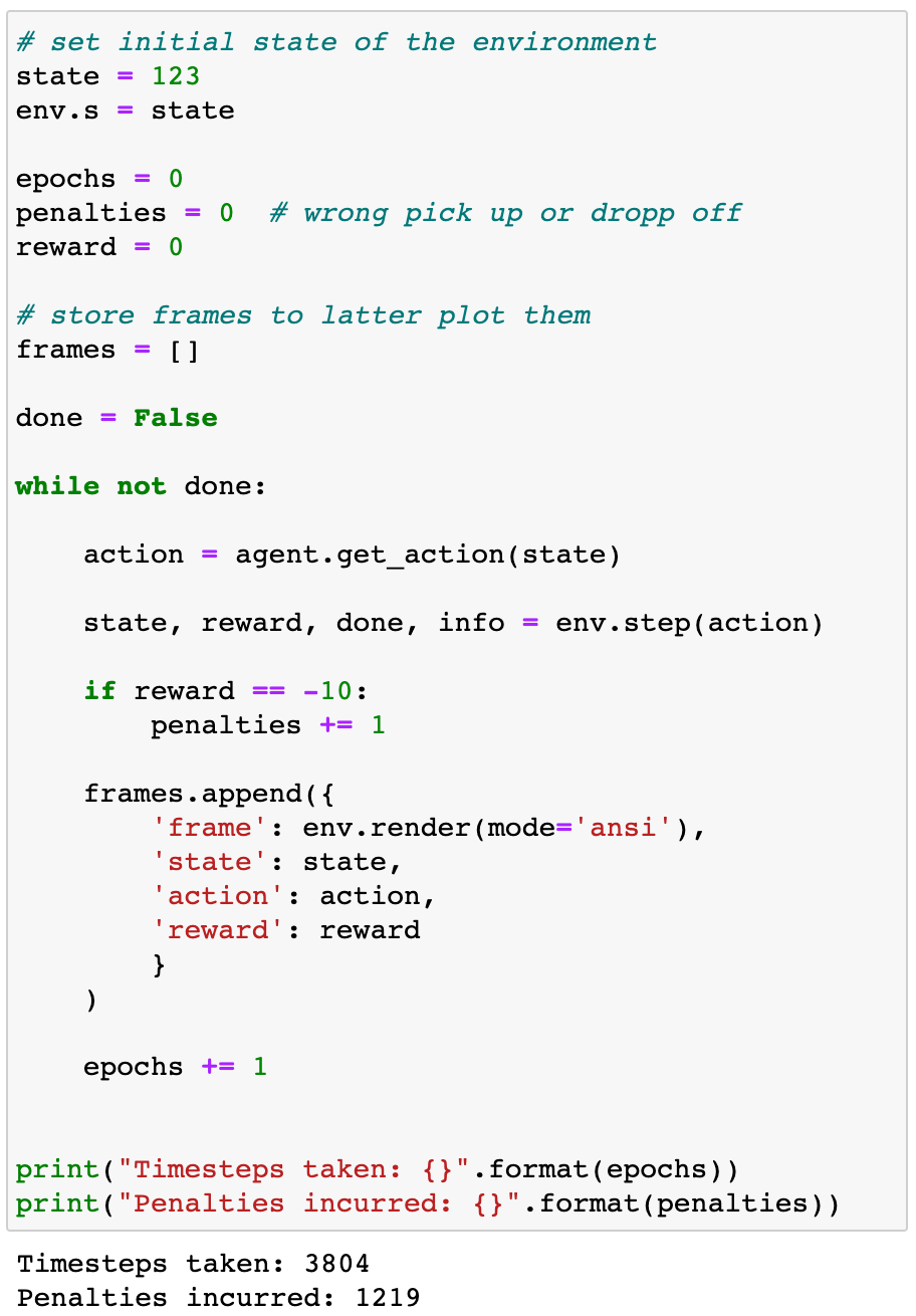
3,804 steps is a lot!
Please watch it yourself in this video:
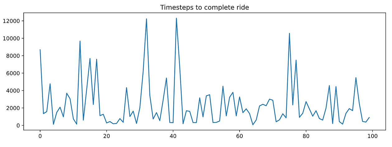
To get a more representative measure of performance, we can repeat the same evaluation loop n=100 times starting each time at a random state.
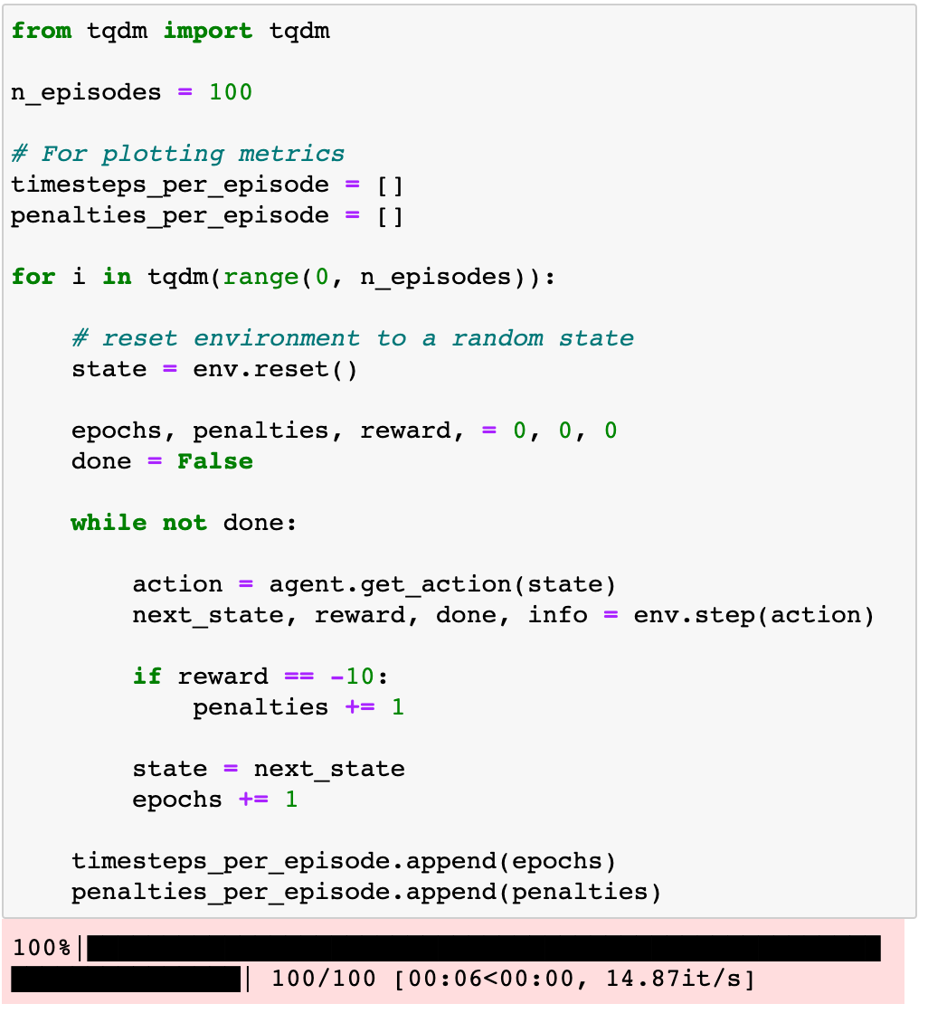
If you plot timesteps_per_episode and penalties_per_episode you can observe that none of them decreases as the agent completes more episodes. In other words, the agent is NOT LEARNING anything.
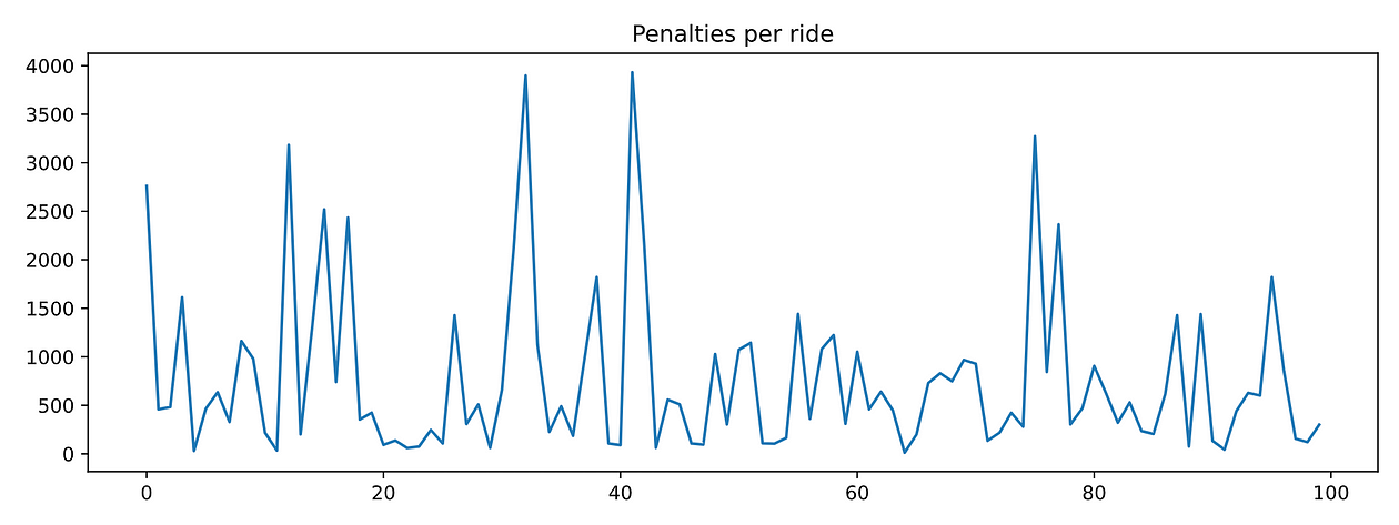
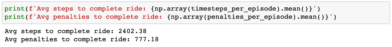
If you want summary statistics of performance, you can take averages:
Implementing agents that learn is the goal of Reinforcement Learning, and of this course too.
Let’s implement our first “intelligent” agent using Q-learning, one of the earliest and most used RL algorithms that exist.
4. Q-learning agent
Q-learning (by Chris Walkins and Peter Dayan) is an algorithm to find the optimal q-value function.
As we said in part 1, the q-value function Q(s, a) associated with a policy π is the total reward the agent expects to get when at state s the agent takes action a and follows policy π thereafter.
The optimal q-value function Q*(s, a)is the q-value function associated with the optimal policy π*.
If you know Q*(s, a), you can infer π*: i.e., you pick as the next action the one that maximizes Q*(s, a) for the current state s.
Q-learning is an iterative algorithm to compute better and better approximations to the optimal q-value function Q*(s, a), starting from an arbitrary initial guess Q⁰(s, a).

In a tabular environment like Taxi-v3 with a finite number of states and actions, a q-function is essentially a matrix. It has as many rows as states and columns as actions, i.e. 500 x 6.
Ok, but how exactly do you compute the next approximation Q¹(s, a) from Q⁰(s, a)?
This is the key formula in Q-learning:
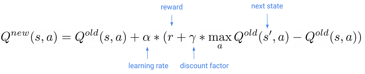
As our q-agent navigates the environment and observes the next state s’ and reward r, you update your q-value matrix with this formula.
What is the learning rate ???? in this formula?
The learning rate (as usual in machine learning) is a small number that controls how large are the updates to the q-function. You need to tune it, as too large of a value will cause unstable training, and too small might not be enough to escape local minima.
And this discount factor ?????
The discount factor is a (hyper) parameter between 0 and 1 that determines how much our agent cares about rewards in the distant future relative to those in the immediate future.
- When ????=0, the agent only cares about maximizing immediate reward. As it happens in life, maximizing immediate reward is not the best recipe for optimal long-term outcomes. This happens in RL agents too.
- When ????=1, the agent evaluates each of its actions based on the sum total of all of its future rewards. In this case, the agent weights equally immediate rewards and future rewards.
The discount factor is typically an intermediate value, e.g., 0.6.
To sum up, if you
- train long enough
- with a decent learning rate and discount factor
- and the agent explores enough the state space
- and you update the q-value matrix with the Q-learning formula,
your initial approximation will eventually converge to optimal q-matrix. Voila!
Let’s implement a Python class for a Q-agent then.
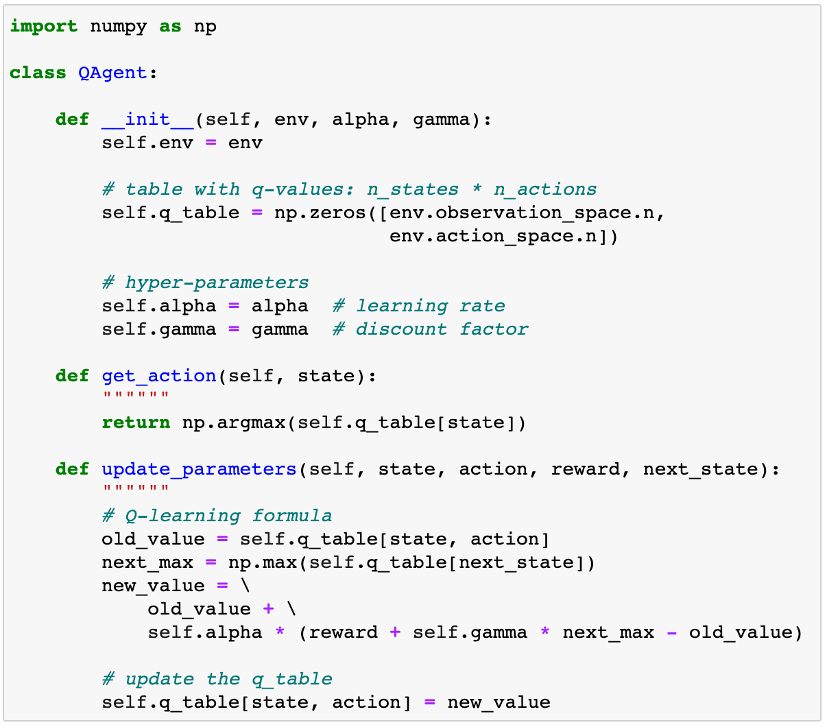
Its API is the same as for the RandomAgent above, but with an extra method update_parameters(). This method takes the transition vector (state, action, reward, next_state) and updates the q-value matrix approximation self.q_table using the Q-learning formula from above.
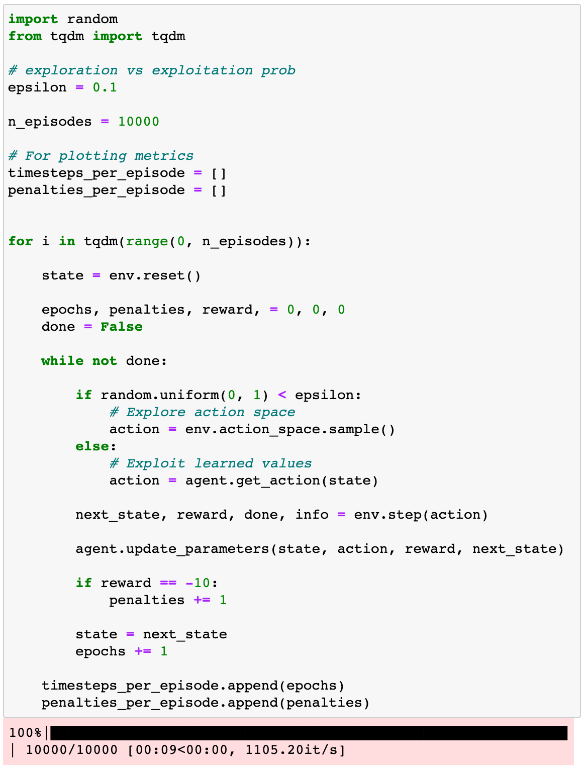
Now, we need to plug this agent into a training loop and call its update_parameters() method every time the agent collects a new experience.
Also, remember we need to guarantee the agent explores enough the state space. Remember the exploration-exploitation parameter we talked about in part 1? This is when the epsilon parameter enters into the game.
Let’s train the agent for n_episodes = 10,000 and use epsilon = 10%:
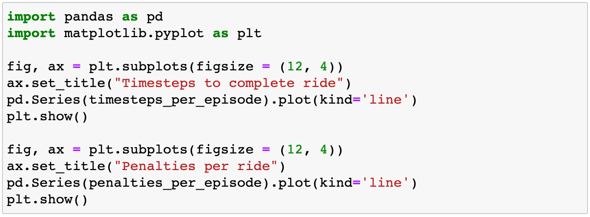
And plot timesteps_per_episode and penalties_per_episode:
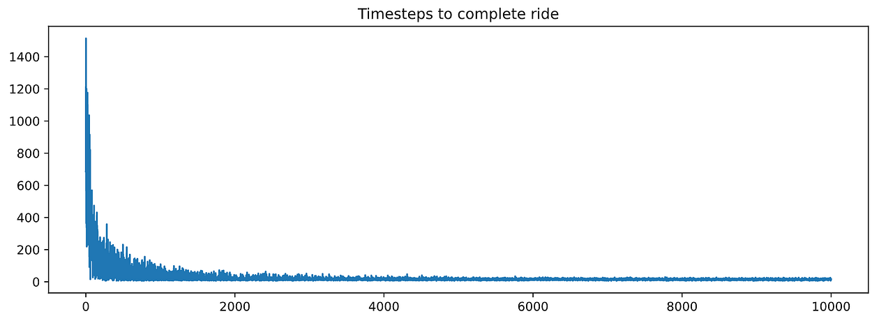
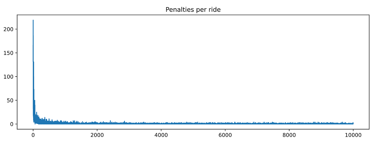
Nice! These graphs look much much better than for the RandomAgent. Both metrics decrease with training, which means our agent is learning.
We can actually see how the agent drives starting from the same state = 123 as we used for the RandomAgent.
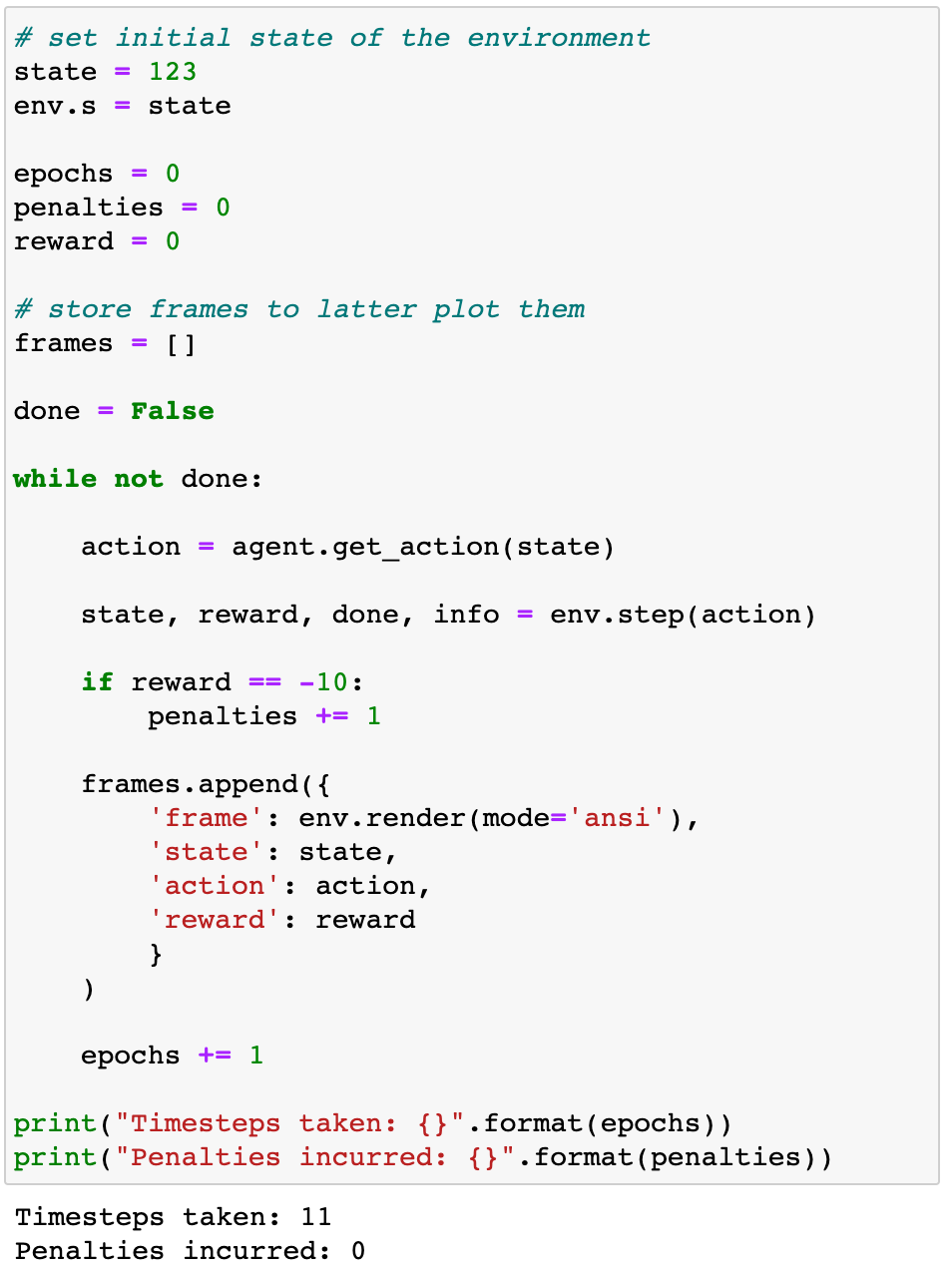
Nice ride by our Q-agent!
If you want to compare hard numbers, you can evaluate the performance of the q-agent on, let’s say, 100 random episodes and compute the average number of timestamps and penalties incurred.
A little bit about epsilon-greedy policies
When you evaluate the agent, it is still good practice to use a positive epsilon value, and not epsilon = 0.
Why so? Isn’t our agent fully trained? Why do we need to keep this source of randomness when we choose the next action?
The reason is to prevent overfitting.
Even for such a small state, action space in Taxi-v3 (i.e., 500 x 6), it is likely that during training, our agent has not visited enough certain states. Hence, its performance in these states might not be 100% optimal, causing the agent to get “caught” in an almost infinite loop of suboptimal actions. If epsilon is a small positive number (e.g., 5%), we can help the agent escape these infinite loops of suboptimal actions.
By using a small epsilon at evaluation, we are adopting a so-called epsilon-greedy strategy.
Let’s evaluate our trained agent on n_episodes = 100 using epsilon = 0.05. Observe how the loop looks almost exactly as the train loop above, but without the call to update_parameters():
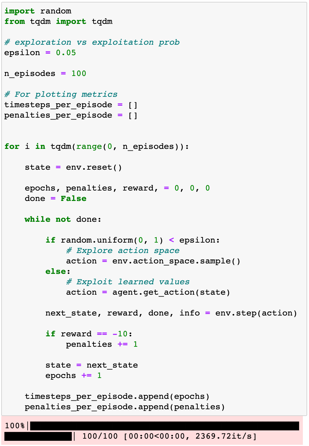
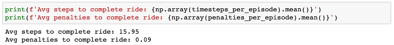
These numbers look much much better than for the RandomAgent.
We can say our agent has learned to drive the taxi!
Q-learning gives us a method to compute optimal q-values. But, what about the hyper-parameters alpha, gamma, and epsilon?
I chose them for you, rather arbitrarily. But in practice, you will need to tune them for your RL problems.
Let’s explore their impact on learning to get a better intuition of what is going on.
5. Hyper-parameter tuning
notebooks/03_q_agent_hyperparameters_analysis.ipynb
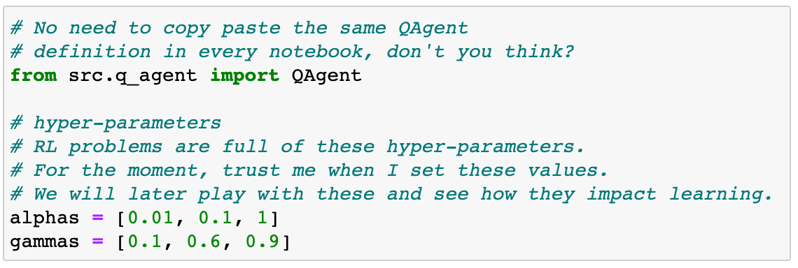
Let’s train our q-agent using different values for alpha (learning rate) and gamma (discount factor). As for epsilon, we keep it at 10%.
In order to keep the code clean, I encapsulated the q-agent definition inside src/q_agent.py and the training loop inside the train() function in src/loops.py.
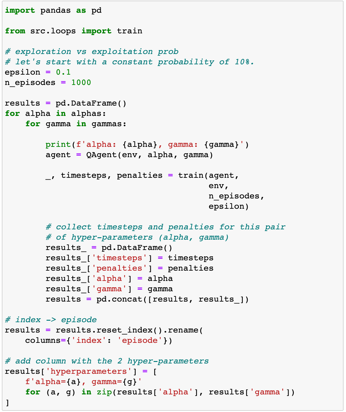
Let us plot the timesteps per episode for each combination of hyper-parameters.
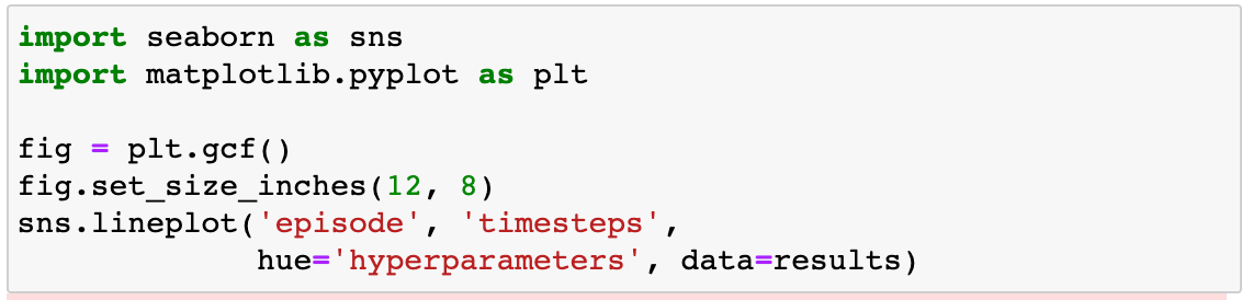
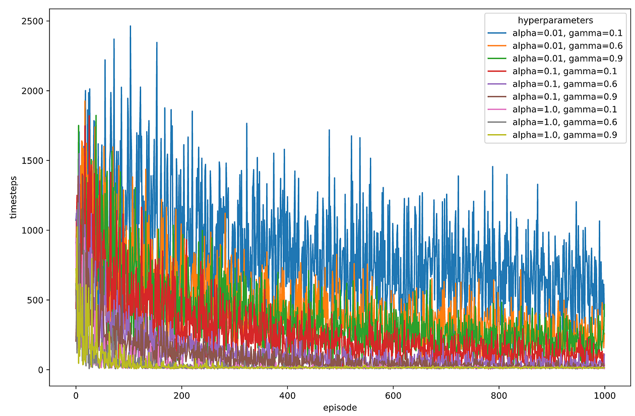
The graph looks artsy but a bit too noisy.
Something you can observe, though, is that when alpha = 0.01 the learning is slower. alpha (learning rate) controls how much we update the q-values in each iteration. Too small of a value implies slower learning.
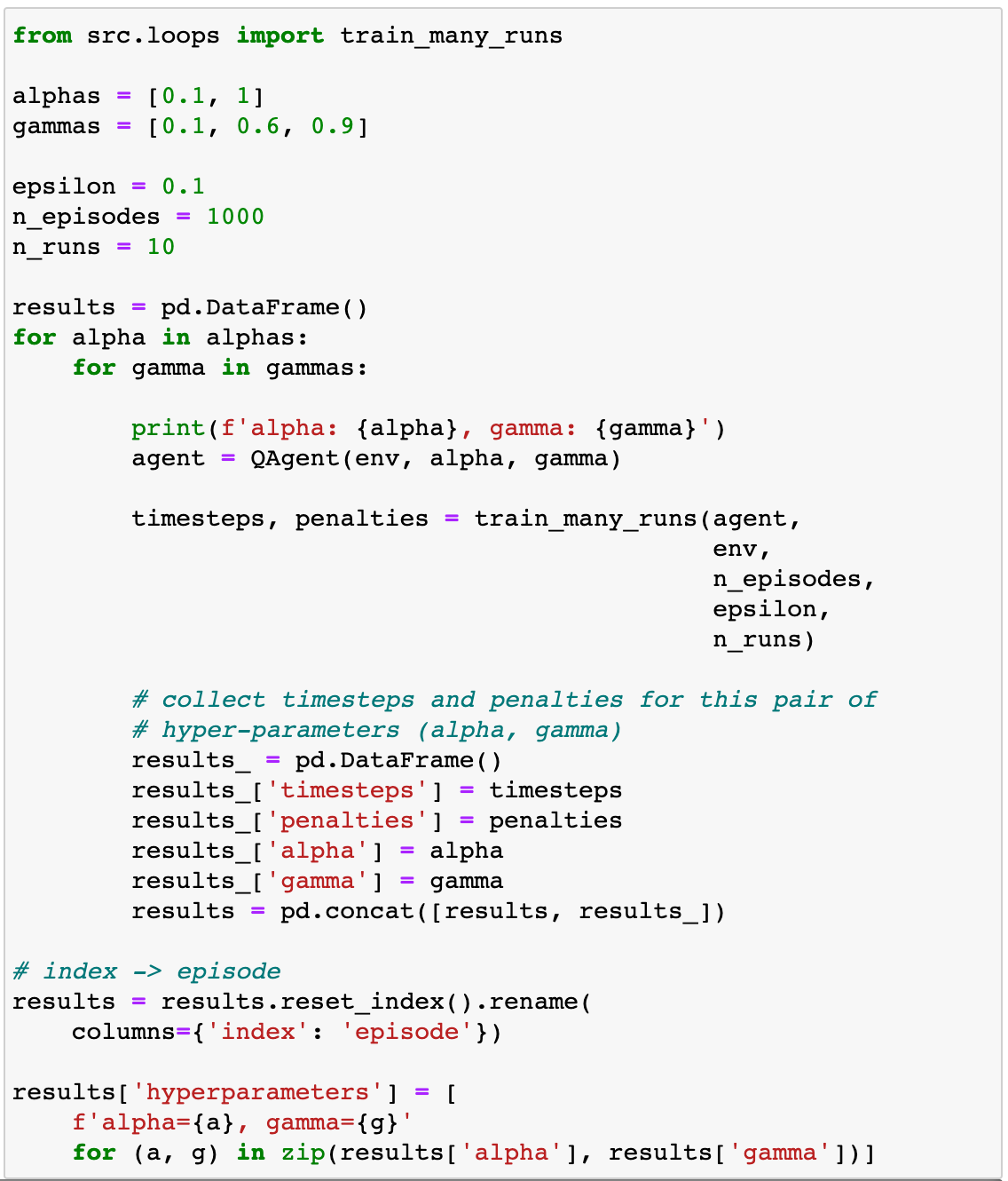
Let’s discard alpha = 0.01 and do 10 runs of training for each combination of hyper-parameters. We average the timesteps for each episode number, from 1 to 1000, using these 10 runs.
I created the function train_many_runs() in src/loops.py to keep the notebook code cleaner:
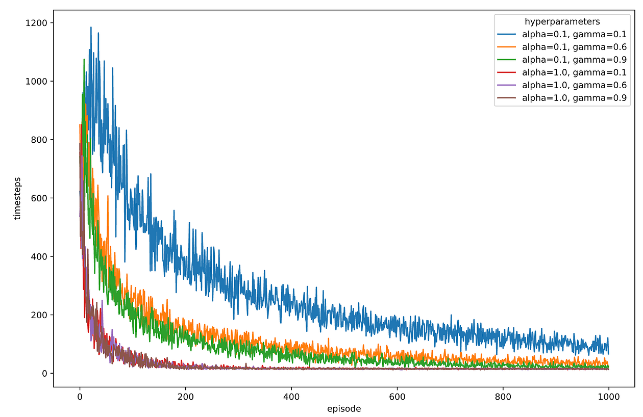
It looks like alpha = 1.0 is the value that works best, while gamma seems to have less of an impact.
Congratulations! You have tuned your first learning rate in this course.
Tuning hyper-parameters can be time-consuming and tedious. There are excellent libraries to automate the manual process we just followed, like Optuna, but this is something we will play with later in the course. For the time being, enjoy the speed-up in training we have just found.
Wait, what happens with this epsilon = 10% that I told you to trust me on?
Is the current 10% value the best?
Let’s check it ourselves.
We take the best alpha and gamma we found, i.e.,
- alpha = 1.0
- gamma = 0.9 (we could have taken 0.1 or 0.6 too)
And train with different epsilons = [0.01, 0.1, 0.9]
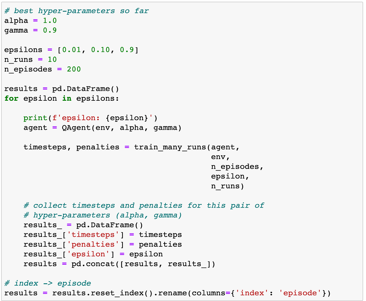
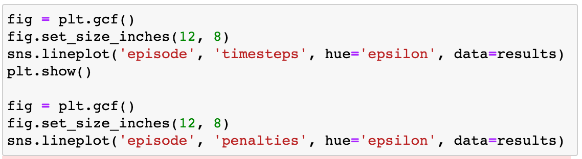
And plot the resulting timesteps and penalties curves:
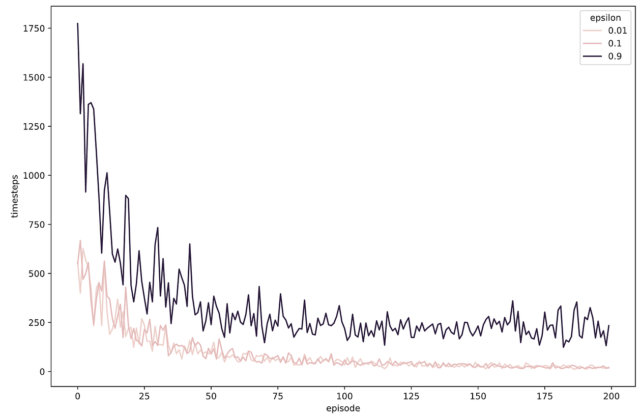
As you can see, both epsilon = 0.01 and epsilon = 0.1 seem to work equally well, as they strike the right balance between exploration and exploitation.
On the other side, epsilon = 0.9 is too large of a value, causing “too much” randomness during training and preventing our q-matrix from converging to the optimal one. Observe how the performance plateaus at around 250 timesteps per episode.
In general, the best strategy to choose the epsilon hyper-parameter is progressive epsilon decay. That is, at the beginning of training, when the agent is very uncertain about its q-value estimation, it is best to visit as many states as possible, and for that, a large epsilon is great (e.g., 50%)
As training progresses and the agent refines its q-value estimation, it is no longer optimal to explore that much. Instead, by decreasing epsilon, the agent can learn to perfect and fine-tune the q-values to make them converge faster to the optimal ones. Too large of epsilon can cause convergence issues, as we see for epsilon = 0.9.
We will be tunning epsilons along the course, so I will not insist too much for the moment. Again, enjoy what we have done today. It is pretty remarkable.

B-R-A-V-O! (Image by the author).
Recap
Congratulations on (probably) solving your first Reinforcement Learning problem.
These are the key learnings I want you to sleep on:
- The difficulty of a Reinforcement Learning problem is directly related to the number of possible actions and states. Taxi-v3 is a tabular environment (i.e. finite number of states and actions), so it is an easy one.
- Q-learning is a learning algorithm that works excellent for tabular environments.
- No matter what RL algorithm you use, there are hyper-parameters you need to tune to make sure your agent learns the optimal strategy.
- Tunning hyper-parameters is a time-consuming process but necessary to ensure our agents learn. We will get better at this as the course progresses.
Homework
This is what I want you to do:
- Git clone the repo to your local machine.
- Setup the environment for this lesson 01_taxi.
- Open 01_taxi/otebooks/04_homework.ipynb and try completing the 2 challenges.
I call them challenges (not exercises) because they are not easy. I want you to try them, get your hands dirty, and (maybe) succeed.
In the first challenge, I dare you to update the train()function src/loops.py to accept an episode-dependent epsilon.
In the second challenge, I want you to upgrade your Python skills and implement paralleling processing to speed up hyper-parameter experimentation.
As usual, if you get stuck and you need feedback, drop me a line at plabartabajo@gmail.com.
I will be more than happy to help you.
If you want to get updates on the course, subscribe to the datamachines newsletter.
Original. Reposted with permission.