7 More Steps to Mastering Machine Learning With Python

Step 4: More Ensemble Methods

 
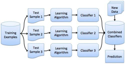
The first post only dealt with a single ensemble method: Random Forests (RF). RF has seen a great deal of success over the years as a top performing classifier, but it is certainly not the only ensemble classifier available. We will have a look at bagging, boosting, and voting.

Give me a boost.

First, read these overviews of ensemble learners, the first being general, and the second being as they relate to Scikit-learn:

• An Introduction to Ensemble Learners, by Matthew Mayo
• Ensemble methods in Scikit-learn, Scikit-learn documentation

Then, before moving on to new ensemble methods, get back up to speed on Random Forests with a fresh tutorial here:

• Random Forests in Python, from Yhat

Bagging, boosting, and voting are all different forms of ensemble classifiers. All involve building multiple models; however, what algorithms the models are built from, the data which the models use, and how the results are ultimately combined differ between schemes.

• Bagging builds multiple models from the same classification algorithm, while using different (independent) samples of data from the training set -- Scikit-learn implements BaggingClassifier
• Boosting builds multiple models from the same classification algorithm, chaining models one after another in order to boost the learning of each subsequent model -- Scikit-learn implements AdaBoost
• Voting builds multiple models from different classification algorithms, and a criteria is used to determine how the models are best combined -- Scikit-learn implements VotingClassifier

So, why combine models? To approach this question from one specific angle, here is an overview of the bias-variance trade-off as related specifically to boosting, from the Scikit-learn documentation:

• Single estimator versus bagging: bias-variance decomposition, Scikit-learn documentation

Now that you have read some introductory material on ensemble learners in general, and have a basic understanding of a few specific ensemble classifiers, follow this introduction to implementing the ensemble classifiers in Python using Scikit-learn, from Machine Learning Mastery:

• Ensemble Machine Learning Algorithms in Python with scikit-learn, by Jason Brownlee

Step 5: Gradient Boosting

 
Our next step keeps us in the realm of ensemble classifiers, focusing on one of the most popular contemporary machine learning algorithms. Gradient boosting has made a noticeable impact in machine learning in the recent past, becoming (of note) one of the most utilized and successful algorithms in Kaggle competitions.

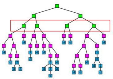
Give me a gradient boost.

First, read an overview of what gradient boosting is:

• Gradient boosting on Wikipedia

Next, read up on why gradient boosting is the "most winning-est" approach to Kaggle competitions:

• Why does Gradient boosting work so well for so many Kaggle problems? on Quora
• A Kaggle Master Explains Gradient Boosting, by Ben Gorman

While Scikit-learn has its own gradient boosting implementation, we will diverge somewhat and use the XGBoost library, which has been noted to be a faster implementation.

The following links provide some additional info on the XGBoost library, as well as gradient boosting (out of necessity):

• XGBoost on Wikipedia
• XGBoost library on Github
• XGBoost documentation

Now, follow this tutorial which brings it all together:

• A Guide to Gradient Boosted Trees with XGBoost in Python, by Jesse Steinweg-Woods

You can also follow these more concise examples for reinforcement:

• XGBoost Example (Python) on Kaggle
• Iris Dataset and XGBoost Simple Tutorial, by Ieva Zarina

Step 6: More Dimensionality Reduction

 
Dimensionality reduction is the act of reducing the variables being used for model building from its initial number to a reduced number, by utilizing processes to obtain a set of principal variables.

There are 2 major forms of dimensionality reduction:

1. Feature selection - selecting a subset of relevant features
2. Feature extraction - building an informative and non-redundant set of derived values features

The following is a look at a pair of common feature extraction methods.

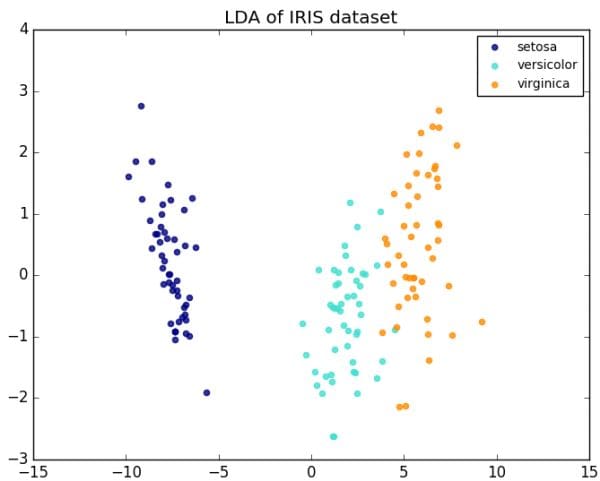
LDA of Iris dataset.

Principal component analysis (PCA) is a statistical procedure that uses an orthogonal transformation to convert a set of observations of possibly correlated variables into a set of values of linearly uncorrelated variables called principal components. The number of principal components is less than or equal to the number of original variables. This transformation is defined in such a way that the first principal component has the largest possible variance (that is, accounts for as much of the variability in the data as possible)[.]

The above definition comes from the PCA Wikipedia entry, which you can read further if interested. However, the following overview-slash-tutorial is very thorough:

• Principal Component Analysis in 3 Simple Steps, by Sebastian Raschka

Linear discriminant analysis (LDA) is a generalization of Fisher's linear discriminant, a method used in statistics, pattern recognition and machine learning to find a linear combination of features that characterizes or separates two or more classes of objects or events. The resulting combination may be used as a linear classifier, or, more commonly, for dimensionality reduction before later classification.

LDA is closely related to analysis of variance (ANOVA) and regression analysis, which also attempt to express one dependent variable as a linear combination of other features or measurements. However, ANOVA uses categorical independent variables and a continuous dependent variable, whereas discriminant analysis has continuous independent variables and a categorical dependent variable (i.e. the class label)

The above definition is also from Wikipedia. And again, the following read is thorough:

• Linear Discriminant Analysis – Bit by Bit, by Sebastian Raschka

Are you at all confused as to the practical difference between PCA and LDA for dimensionality reduction? Sebastian Raschka clarifies:

Both Linear Discriminant Analysis (LDA) and Principal Component Analysis (PCA) are linear transformation techniques that are commonly used for dimensionality reduction. PCA can be described as an “unsupervised” algorithm, since it “ignores” class labels and its goal is to find the directions (the so-called principal components) that maximize the variance in a dataset. In contrast to PCA, LDA is “supervised” and computes the directions (“linear discriminants”) that will represent the axes that that maximize the separation between multiple classes.

For a concise elaboration on this, read the following:

• What is the difference between LDA and PCA for dimensionality reduction?, by Sebastian Raschka

Step 7: More Deep Learning

 
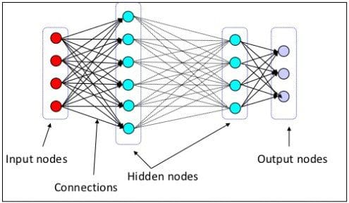
The original 7 Steps... post provided an entry point to neural networks and deep learning. If you have made it this far without much trouble and want to solidify your understanding of neural networks, and practice implementing a few common neural network models, there is no reason not to continue on.

The many layers of deep neural networks.

First, have a look at a few deep learning foundation materials:

• Deep Learning Key Terms, Explained, by Matthew Mayo
• 7 Steps to Understanding Deep Learning, by Matthew Mayo

Next, try a few introductory overview-slash-tutorials on TensorFlow, Google's "open-source software library for Machine Intelligence," effectively a deep learning framework and nearly de facto contemporary go-to neural network tool:

• The Gentlest Introduction to Tensorflow – Part 1, by Soon Hin Khor
• The Gentlest Introduction to Tensorflow – Part 2, by Soon Hin Khor
• The Gentlest Introduction to Tensorflow – Part 3, by Soon Hin Khor
• The Gentlest Introduction to Tensorflow – Part 4, by Soon Hin Khor

Finally, try your hand at these tutorials directly from the TensorFlow site, which implement a few of the most popular and common neural network models:

• Recurrent Neural Networks, Google TensorFlow tutorial
• Convolutional Neural Networks, Google TensorFlow tutorial

Also, a 7 Steps... post focusing on deep learning is currently in the works, and will focus on the use of a high-level API sitting atop TensorFlow to increase the ease and flexibility with which a practitioner can implement models. I will also add a link here once complete.

Related:

• 5 EBooks to Read Before Getting into A Machine Learning Career
• 7 Steps to Understanding Deep Learning
• Machine Learning Key Terms, Explained