Keras Tutorial: Recognizing Tic-Tac-Toe Winners with Neural Networks
In this tutorial, we will build a neural network with Keras to determine whether or not tic-tac-toe games have been won by player X for given endgame board configurations. Introductory neural network concerns are covered.

"Tic-Tac-Toe Endgame" was the very first dataset I used to build a neural network some years ago. I didn't really know what I was doing at the time, and so things didn't go so well. As I have been spending a lot of time with Keras recently, I thought I would take another stab at this dataset in order to demonstrate building a simple neural network with Keras.
The Data
The dataset, available here, is a collection of 958 possible tac-tac-toe end-of-game board configurations, with 9 variables representing the 9 squares of a tic-tac-toe board, and a tenth class variable which designates if the described board configuration is a winning (positive) or not (negative) ending configuration for player X. In short, does a particular collection of Xs and Os on a board mean a win for X? Incidentally, there are 255,168 possible ways of playing a game of tic-tac-toe.
Here is a more formal description of the data:
1. top-left-square: {x,o,b}
2. top-middle-square: {x,o,b}
3. top-right-square: {x,o,b}
4. middle-left-square: {x,o,b}
5. middle-middle-square: {x,o,b}
6. middle-right-square: {x,o,b}
7. bottom-left-square: {x,o,b}
8. bottom-middle-square: {x,o,b}
9. bottom-right-square: {x,o,b}
10. Class: {positive,negative}
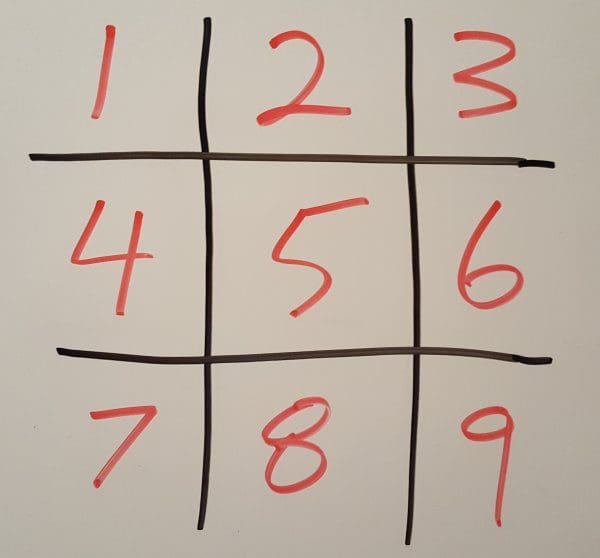
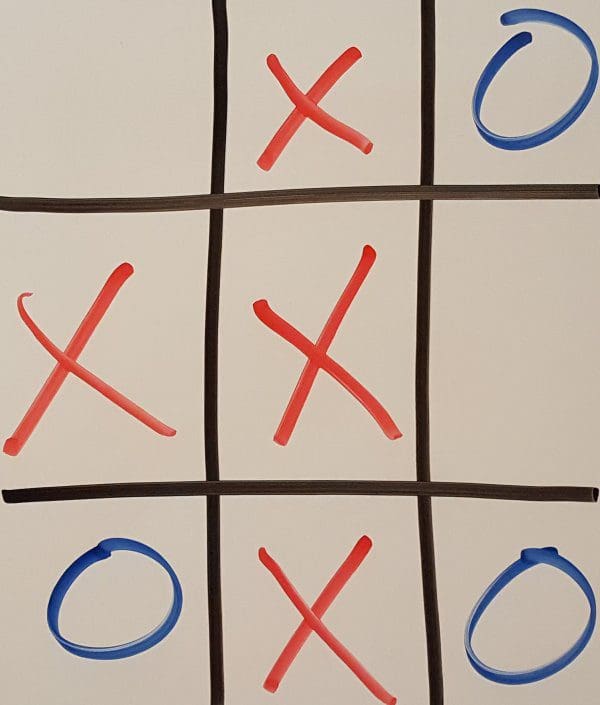
As is visible, each square can be designated as marked with an X, an O, or left blank (b) at game's end. The mapping of variables to physical squares is shown in Figure 1. Remember, the outcomes are positive or negative based on X winning. Figure 2 portrays a example board endgame layout, followed by its dataset representation.

Figure 1. Mapping of variables to physical tic-tac-toe board locations.

Figure 2. Example board endgame layout.
b,x,o,x,x,b,o,x,o,positive
The Preparation
In order to use the dataset to construct a neural network, some data preparation and transformations will be necessary. These are outlined below, as well as further commented upon in the code further down.
- Encode categorical variables as numeric - Each square is represented as a single variable in the original dataset. This is unacceptable for our purposes, however, as neural networks require variables with continuous values. We must first convert {x, o, b} to {0, 1, 2} for each variable. The LabelEncoder class of Scikit-learn preprocessing module will be used to accomplish this.
- One-hot encode all independent categorical variables - Once categorical variables are encoded to numeric, they required further processing. As the variables are unordered (X is not greater than O, for example), these variables must be represented as a series of bit equivalents. This is accomplished using one-hot encoding. As there are 3 possibilities for each square, 2 bits will be required for encoding. This will be accomplished with the OneHotEncoder class from Scikit-learn.
- Remove every third column to avoid dummy variable trap - As the one-hot encoding process in Scikit-learn creates as many columns for each variables as there are possible options (as per the dataset), one column needs to be removed in order to avoid what is referred to as the dummy variable trap. This is so to avoid redundant data which could bias results. In our case, each square has 3 possible options (27 columns), which can be expressed with 2 'bit' columns (I leave this to you to confirm), and so we remove every third column from the newly formed dataset (leaving us with 18).
- Encode target categorical variable - Similarly to the independent variables, the target categorical variable must be changed from {positive, negative} to {0, 1}.
- Train/test split - This should be understandable to all. We set our test set to 20% of the dataset. We will use Scikit-learn's train/test split functionality to achieve this.
The Network
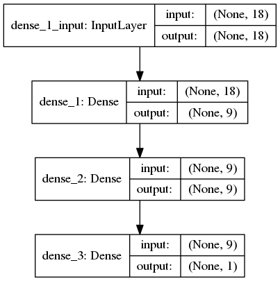
Next, we need to construct the neural network, which we will do using Keras. Let's keep in mind that our processed dataset has 18 variables to use as input, and that we are making binary class predictions as output.
- Input neurons - We have 18 independent variables; therefore, we need 18 input neurons.
- Hidden layers - A simple (perhaps overly so) -- and possibly totally nonsensical -- starting point to determining the number of neurons per hidden layer is the rule of thumb: add the number of independent variables and the number of output variables and divide by 2. If we decide to round down, this gives us 9. What about the number of hidden layers? Best idea is to start with a low number (of hidden layers) and add them until network accuracy does not improve. We will create our network with 2 hidden layers.
- Activation functions - Hidden and output layer neurons require activation functions. General rules dictate: hidden layer neurons get the ReLU function by default, while binary classification output layer neurons get the sigmoid function. We will follow convention.
- Optimizer - We will use the Adam optimizer in our network
- Loss function - We will use the cross-entropy loss function in our network.
- Weight initialization - We will randomly set the initial random weights of our network layer neurons.
Below is what our network will ultimately look like.

Figure 3. Visualization of network layers.
The Code
Here is the code which does everything outlined above.
The Results
The maximum accuracy of the trained network reached 98.69%. On the unseen test set, the neural network correctly predicted the class of 180 of the 186 instances.
By changing the random state of the train/test split (which changes which particular 20% of dataset instances are used to test the resultant network with), we were able to increase this to 184 out of 186 instances. This is not necessarily a true metric improvement, however. An independent verification set could possibly shed light on this... if we had one.
By using different optimizers (as opposed to Adam), a well as changing the number of hidden layers and the number of neurons per hidden layer, the resulting trained networks did not result in better loss, accuracy, or correctly classified test instances beyond what is reported above.
I hope this has been a useful introduction to constructing neural networks with Keras. The next such tutorial will attack convolutional neural network construction.
Related:
