Understanding Feature Engineering: Deep Learning Methods for Text Data
Newer, advanced strategies for taming unstructured, textual data: In this article, we will be looking at more advanced feature engineering strategies which often leverage deep learning models.
Editor's note: This post is only one part of a far more thorough and in-depth original, found here, which covers much more than what is included here.

Introduction
Working with unstructured text data is hard especially when you are trying to build an intelligent system which interprets and understands free flowing natural language just like humans. You need to be able to process and transform noisy, unstructured textual data into some structured, vectorized formats which can be understood by any machine learning algorithm. Principles from Natural Language Processing, Machine Learning or Deep Learning all of which fall under the broad umbrella of Artificial Intelligence are effective tools of the trade. Based on my previous posts, an important point to remember here is that any machine learning algorithm is based on principles of statistics, math and optimization. Hence they are not intelligent enough to start processing text in their raw, native form. We covered some traditional strategies for extracting meaningful features from text data in Part-3: Traditional Methods for Text Data. I encourage you to check out the same for a brief refresher. In this article, we will be looking at more advanced feature engineering strategies which often leverage deep learning models. More specifically we will be covering the Word2Vec, GloVe and FastText models.
Motivation
We have discussed time and again including in our previous article that Feature Engineering is the secret sauce to creating superior and better performing machine learning models. Always remember that even with the advent of automated feature engineering capabilities, you would still need to understand the core concepts behind applying the techniques. Otherwise they would just be black box models which you wouldn’t know how to tweak and tune for the problem you are trying to solve.
Shortcomings of traditional models
Traditional (count-based) feature engineering strategies for textual data involve models belonging to a family of models popularly known as the Bag of Words model. This includes term frequencies, TF-IDF (term frequency-inverse document frequency), N-grams and so on. While they are effective methods for extracting features from text, due to the inherent nature of the model being just a bag of unstructured words, we lose additional information like the semantics, structure, sequence and context around nearby words in each text document. This forms as enough motivation for us to explore more sophisticated models which can capture this information and give us features which are vector representation of words, popularly known as embeddings.
The need for word embeddings
While this does make some sense, why should we be motivated enough to learn and build these word embeddings? With regard to speech or image recognition systems, all the information is already present in the form of rich dense feature vectors embedded in high-dimensional datasets like audio spectrograms and image pixel intensities. However when it comes to raw text data, especially count based models like Bag of Words, we are dealing with individual words which may have their own identifiers and do not capture the semantic relationship amongst words. This leads to huge sparse word vectors for textual data and thus if we do not have enough data, we may end up getting poor models or even overfitting the data due to the curse of dimensionality.
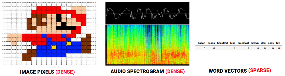
Comparing feature representations for audio, image and text
Feature Engineering Strategies
Let’s look at some of these advanced strategies for handling text data and extracting meaningful features from the same, which can be used in downstream machine learning systems. Do note that you can access all the code used in this article in my GitHub repository also for future reference. We’ll start by loading up some basic dependencies and settings.
import pandas as pd
import numpy as np
import re
import nltk
import matplotlib.pyplot as plt

pd.options.display.max_colwidth = 200
%matplotlib inline
We will now take a few corpora of documents on which we will perform all our analyses. For one of the corpora, we will reuse our corpus from our previous article, Part-3: Traditional Methods for Text Data. We mention the code as follows for ease of understanding.

Our sample text corpus
corpus module in nltk. We will load this up shortly, in the next section. Before we talk about feature engineering, we need to pre-process and normalize this text.
Text pre-processing
There can be multiple ways of cleaning and pre-processing textual data. The most important techniques which are used heavily in Natural Language Processing (NLP) pipelines have been highlighted in detail in the ‘Text pre-processing’ section in Part 3 of this series. Since the focus of this article is on feature engineering, just like our previous article, we will re-use our simple text pre-processor which focuses on removing special characters, extra whitespaces, digits, stopwords and lower casing the text corpus.
Once we have our basic pre-processing pipeline ready, let’s first apply the same to our toy corpus.
norm_corpus = normalize_corpus(corpus)
norm_corpus

Output
------
array(['sky blue beautiful', 'love blue beautiful sky',
       'quick brown fox jumps lazy dog',
       'kings breakfast sausages ham bacon eggs toast beans',
       'love green eggs ham sausages bacon',
       'brown fox quick blue dog lazy',
       'sky blue sky beautiful today',
       'dog lazy brown fox quick'],
      dtype='<U51')
Let’s now load up our other corpus based on The King James Version of the Bible using nltk and pre-process the text.
The following output shows the total number of lines in our corpus and how the pre-processing works on the textual content.
Output
------

Total lines: 30103

Sample line: ['1', ':', '6', 'And', 'God', 'said', ',', 'Let', 'there', 'be', 'a', 'firmament', 'in', 'the', 'midst', 'of', 'the', 'waters', ',', 'and', 'let', 'it', 'divide', 'the', 'waters', 'from', 'the', 'waters', '.']

Processed line: god said let firmament midst waters let divide waters waters
Bio: Dipanjan Sarkar is a Data Scientist @Intel, an author, a mentor @Springboard, a writer, and a sports and sitcom addict.
Original. Reposted with permission.
Related: