Implementing Deep Learning Methods and Feature Engineering for Text Data: FastText

comments

Editor's note: This post is only one part of a far more thorough and in-depth original, found here, which covers much more than what is included here.

The FastText Model

 
The FastText model was first introduced by Facebook in 2016 as an extension and supposedly improvement of the vanilla Word2Vec model. Based on the original paper titled ‘Enriching Word Vectors with Subword Information’ by Mikolov et al. which is an excellent read to gain an in-depth understanding of how this model works. Overall, FastText is a framework for learning word representations and also performing robust, fast and accurate text classification. The framework is open-sourced by Facebook on GitHub and claims to have the following.

• Recent state-of-the-art English word vectors.
• Word vectors for 157 languages trained on Wikipedia and Crawl.
• Models for language identification and various supervised tasks.

Though I haven’t implemented this model from scratch, based on the research paper, following is what I learnt about how the model works. In general, predictive models like the Word2Vec model typically considers each word as a distinct entity (e.g. where) and generates a dense embedding for the word. However this poses to be a serious limitation with languages having massive vocabularies and many rare words which may not occur a lot in different corpora. The Word2Vec model typically ignores the morphological structure of each word and considers a word as a single entity. The FastText model considers each word as a Bag of Character n-grams. This is also called as a subword model in the paper.

We add special boundary symbols < and > at the beginning and end of words. This enables us to distinguish prefixes and suffixes from other character sequences. We also include the word w itself in the set of its n-grams, to learn a representation for each word (in addition to its character n-grams). Taking the word where and n=3 (tri-grams) as an example, it will be represented by the character n-grams: <wh, whe, her, ere, re> and the special sequence <where> representing the whole word. Note that the sequence , corresponding to the word <her> is different from the tri-gram her from the word where.

In practice, the paper recommends in extracting all the n-grams for n ≥ 3 and n ≤ 6. This is a very simple approach, and different sets of n-grams could be considered, for example taking all prefixes and suffixes. We typically associate a vector representation (embedding) to each n-gram for a word. Thus, we can represent a word by the sum of the vector representations of its n-grams or the average of the embedding of these n-grams. Thus, due to this effect of leveraging n-grams from individual words based on their characters, there is a higher chance for rare words to get a good representation since their character based n-grams should occur across other words of the corpus.

Applying FastText features for Machine Learning Tasks

 
The gensim package has nice wrappers providing us interfaces to leverage the FastText model available under the gensim.models.fasttext module. Let’s apply this once again on our Bible corpus and look at our words of interest and their most similar words.

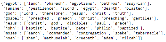
You can see a lot of similarity in the results with our Word2Vec model with relevant similar words for each of our words of interest. Do you notice any interesting associations and similarities?

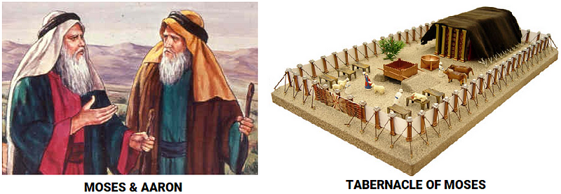
Moses, his brother Aaron and the Tabernacle of Moses

Note: Running this model is computationally expensive and usually takes more time as compared to the skip-gram model since it considers n-grams for each word. This works better if trained using a GPU or a good CPU. I trained this on an AWS p2.x instance and it took me around 10 minutes as compared to over 2–3 hours on a regular system.

Let’s now use Principal Component Analysis (PCA) to reduce the word embedding dimensions to 2-D and then visualize the same.

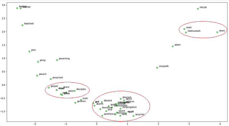
Visualizing FastTest word embeddings on our Bible corpus

We can see a lot of interesting patterns! Noah, his son Shem and grandfather Methuselah are close to each other. We also see God associated with Moses and Egypt where it endured the Biblical plagues including famine and pestilence. Also Jesus and some of his disciples are associated close to each other.

To access any of the word embeddings you can just index the model with the word as follows.

ft_model.wv['jesus']

array([-0.23493268,  0.14237943,  0.35635167,  0.34680951,    
        0.09342121,..., -0.15021783, -0.08518736, -0.28278247,   
       -0.19060139], dtype=float32)

Having these embeddings, we can perform some interesting natural language tasks. One of these would be to find out similarity between different words (entities).

print(ft_model.wv.similarity(w1='god', w2='satan'))
print(ft_model.wv.similarity(w1='god', w2='jesus'))

Output
------
0.333260876685
0.698824900473

We can see that ‘god’ is more closely associated with ‘jesus’ rather than ‘satan’ based on the text in our Bible corpus. Quite relevant!

Considering word embeddings being present, we can even find out odd words from a bunch of words as follows.

st1 = "god jesus satan john"
print('Odd one out for [',st1, ']:',  
      ft_model.wv.doesnt_match(st1.split()))

st2 = "john peter james judas"
print('Odd one out for [',st2, ']:', 
      ft_model.wv.doesnt_match(st2.split()))

Output
------
Odd one out for [ god jesus satan john ]: satan
Odd one out for [ john peter james judas ]: judas

Interesting and relevant results in both cases for the odd entity amongst the other words!

Conclusion

 
These examples should give you a good idea about newer and efficient strategies around leveraging deep learning language models to extract features from text data and also address problems like word semantics, context and data sparsity. Next up will be detailed strategies on leveraging deep learning models for feature engineering on image data. Stay tuned!

To read about feature engineering strategies for continuous numeric data, check out Part 1 of this series!

To read about feature engineering strategies for discrete categoricial data, check out Part 2 of this series!

To read about traditional feature engineering strategies for unstructured text data, check out Part 3 of this series!

All the code and datasets used in this article can be accessed from my GitHub

The code is also available as a Jupyter notebook

Architecture diagrams unless explicitly cited are my copyright. Feel free to use them, but please do remember to cite the source if you want to use them in your own work.

If you have any feedback, comments or interesting insights to share about my article or data science in general, feel free to reach out to me on my LinkedIn social media channel.

 
Bio: Dipanjan Sarkar is a Data Scientist @Intel, an author, a mentor @Springboard, a writer, and a sports and sitcom addict.

Original. Reposted with permission.

Related:

• Text Data Preprocessing: A Walkthrough in Python
• A General Approach to Preprocessing Text Data
• A Framework for Approaching Textual Data Science Tasks