Autotuning for Multi-Objective Optimization on LinkedIn’s Feed Ranking

By Marco Varela & Mavis Li, LinkedIn

The mission of LinkedIn’s Feed on the Homepage is to enable members to build an active professional community that advances their careers. In order to provide the best experience on the Feed, we leverage Artificial Intelligence (AI) to show the most relevant content to the members. This is challenging because we need to choose what content to show out of hundreds of options. The content types can range from article shares by other members to job recommendations to course recommendations, and each type has a different way of enriching our ecosystem, which as a whole aim to fulfill LinkedIn’s mission to “connect the world’s professionals to make them more productive and successful”. Given that we want to provide a diverse and rich experience to our members, we cannot simply strive to increase clicks.

In order to achieve the right balance of content for optimal member experience, we follow a multi-objective optimization approach. We have different machine learning models that optimize for different objectives such as reacts, comments, downstream impact from actions. However, the balance of these different objectives has been achieved manually with the adjustment of parameters by machine learning engineers, which is very inefficient.

In this post, we share our experience coming up with an automated system to tune one of the main parameters in our machine learning model that recommends content on LinkedIn’s Feed, which is just one piece of the community-focused architecture. We aim to achieve the right balance of metrics for our members while addressing the productivity of our engineers and meeting constraints in our ecosystem. For additional context on LinkedIn’s feed, please refer to this blog post.

 

Approach to Manage Metrics Trade-offs on Feed

 
In order to address the complexity and tradeoffs in our ecosystem, we optimize for one set of metrics while keeping another set constant. The optimization part comes from our desire to maximize the “contributions” by our members. By “contribution” we mostly refer to likes, comments, and shares, which are actions that are more likely to drive conversations in our ecosystem, as opposed to simple clicks on articles. Contributions drive more conversations in a few ways: shares create new posts on feed, comments enable members to start conversations with post authors, and likes generate downstream updates in the member's network. These actions can be considered “active” in that members actively consume content by contributing to the ecosystem.

However, we also wanted to leave room for content that isn’t as conversation-driven and can be considered more “passive”. In particular, infrequent visitors on Feed are more likely to be involved in passive consumption. Because of these reasons we decided to keep “passive” consumption constant.

 

Translating Metrics Trade-off into a Scoring Function

 
Given the diversity of content and objectives we need to manage on LinkedIn’s Feed, we decided to apply a multi-objective optimization approach to rank content on our feed. At a high level (skipping many details) we score each of our updates roughly with the following equation:

 

 

You can think of each P(x) as the probability score from a model for the particular objective. We use a lever known as the click weight (????) to choose between more passive-consumption content (e.g. job or article recommendations that might drive clicks) vs. more community-driven content (e.g. a post that might encourage comments). Different types of content are better for one use case than the other, so there’s a tradeoff between passive consumption and active consumption. Even within a particular type of content, there can be items that encourage more passive actions compared to active actions. For example, a trending article might just encourage clicks, but an article from a close connection could spark conversations.

 

Why We Need to Constantly Manage Trade-offs

 
Now that we have provided enough context on LinkedIn’s Feed, we’d like to share bits of our journey in choosing the right ???? (click weight) to balance passive consumption (i.e. clicks) vs. active consumption (i.e like, comment, shares). For the rest of the post, we’ll refer to the action set of like, comment, and share as “contributions.”

The ???? parameter determines the balance between active and passive consumption cannot remain static for several reasons. We continuously work on our machine learning models to provide the best experience to our members, which might affect the balance between the two metrics. For example, we may incorporate new features or try new modeling approaches. This affects the balance in several ways. One way is that a particular feature change (e.g. member affinity to article posts) or model change might be better at recommending content for active consumption than passive consumption or vice versa. Another way is that there are random components in our training process that might change the optimal weight after retraining a model.

 

Challenges with Maintaining Balance in a Multi-Objective Environment

 
Our initial approach to manage the right balance was to build an offline simulator based on historical data to run our models and then get simulated metrics on different values of ????. This allowed us to get a sense of the right ???? by looking at output graphs like the following, where each dot represents a different ????:

 

However, this method proved not to be enough. Our simulator approach inherently has limitations in predicting the effect in the online world due to several reasons:

1. The LinkedIn ecosystem changes over time. Perhaps UI changes are introduced that affect member behavior, or maybe we introduce new content to the feed that wasn’t available before, such as polls. These changes are hard to replicate offline since the simulator is limited to historical data and might not fully reflect the current state of the ecosystem.
2. The sequence of actions a member might take could differ depending on the content shown. For example, if they saw an article first they really liked they might be more likely to continue interacting with other updates.
3. There are reinforcement learning components in the ecosystem that are particularly tricky to reflect in a simulator environment.

As a result, machine learning engineers had to launch multiple versions of a model online for live traffic to test out different ???? values, which caused two main pain points. First, it became time-consuming for engineers to create variants with different ???? values of a particular model, especially since the process involved trial and error. Second, given that we rely on A/B experiments to evaluate each variant, we would run out of online traffic and not be able to test as many experiments as we wanted to.

 

New Approach to Choose Trade-off: Online Autotuning

 
Given the difficulties in manually tuning ???? online, we decided to automate the process with the goal of reducing manual engineering work and the online traffic burden. We identified several requirements to allow our team to easily leverage the tool and to allow enough experiments to run at the same time by respecting online traffic needs:

1. The tool needed to be easy to use given that we are trying to remove manual work for engineers, and it should be easily adoptable by tens of machine learning engineers.
2. The tool should only require a small percentage of total traffic. E.g. if the tool takes 50% of traffic it wouldn’t be useful.
3. The tool should conclude on an optimal value for ???? in a relatively short period of time. E.g. if the tool takes a month to find an optimal weight, it’s not useful.

Requirements 2 and 3 are needed to ensure we can maximize the number of experiments run at the same time.

 

Implementation of Online Autotuning: Initial Strategy Overview

 
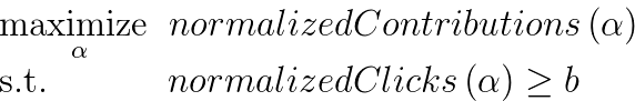
With these requirements in mind, we decided to leverage the TALOS (tuning all large-scale online systems) library within LinkedIn, which is designed to learn parameters in the online setting. Our goal is to autotune the click weight (????) so that we maximize contributions while maintaining the level of passive consumption. Formally, our problem can be written as follows:

 

 

where b is a constant equal to the normalized clicks of the baseline model and ???? is the click weight. We normalized contributions and clicks based on the number of times the Feed was loaded with the relevant alpha (i.e. contributions/loaded_feeds).

Our initial attempt at solving this problem involved using an explore-exploit strategy with TALOS. The explore phase would put members in different click weight buckets and collect relevant metrics (i.e. contributions, normalized click) for a few days. In the exploit phase, the algorithm would zoom in on a click weight range to collect extra data in the range closer to the solution.

 

Implementation of Online Autotuning: Metrics Understanding

 
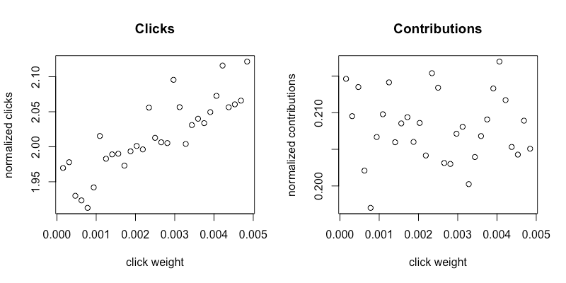
Before we could implement the solution, we first focused on understanding our metrics. This involved determining the grid points and search range of exploration. We chose the search range of exploration based on the manual chosen click weights from historical model iterations, [0.0, 0.005]. There is a tradeoff in choosing the number of grid points. Increasing the number of points gives us more granularity in the click weight, but also gives each point less traffic and hence more noise in the metric. Upon collection of our metrics when ramped with 31 grid points we saw mostly noise with the normalized contributions metric and an increasing trend with the normalized clicks metrics. This is illustrated in figures 2a and 2b, which show the results for an experiment with desktop (non-app) users.

 

To remedy this situation, we did two things:

1. Reduced the number of points, from 31 to 15, to collect more data at each click weight
2. Increased the size of our search range in order to see the relationship between contributions and click weight more clearly

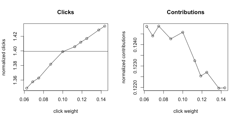
As we can see from figures 3a and 3b, there is a clear trend in both clicks and contributions after the changes.

 

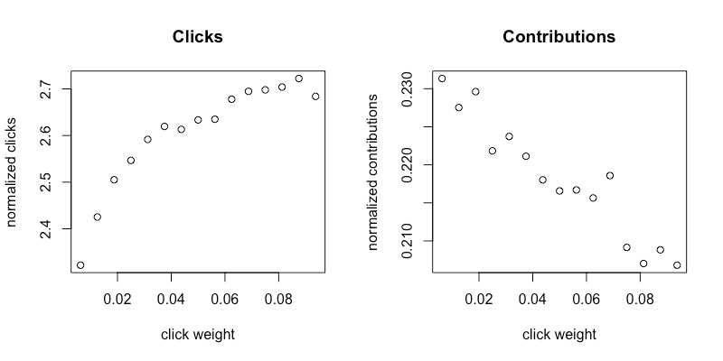
Figures 3a and 3b are the results of reducing points and increasing the search range.

 

Implementation of Online Autotuning: Experience with Initial Strategy

 
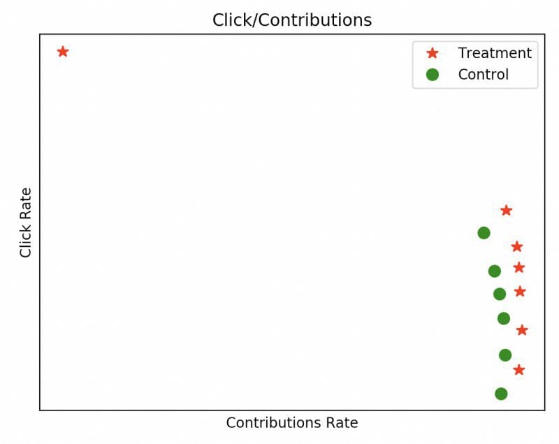
Once we determined the right parameters to reliably capture metrics, we experimented with exploitation, as shown in the graphs below. The search range is different since a different model on a different platform (mobile) is being exemplified in this section.

 

Figures 4a and 4b show metrics collected in the exploration phase. We see a clear positive trend in the normalized clicks metric (4a) and a decreasing but noisy trend in the normalized contributions metric (4b). The black horizontal line is at the constant b, which is the normalized clicks of our control model.

 

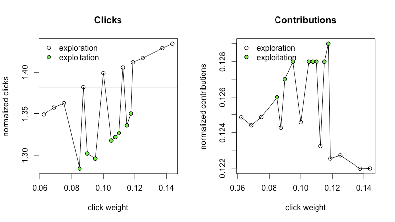
Figures 5a and 5b show an aggregation of metrics over an exploration phase followed by an exploitation phase. The white points are from the exploration phase (same data as in 4a and 4b). After the exploration phase, the algorithm decided the solution was in a reduced search range and selected new points (the green points) to collect metrics for the exploitation phase.

The green exploitation points added too much noise to our metric, making it unclear which click weights were actually feasible. This was surprising, so we looked at our metrics a bit more closely. We first looked at how normalized clicks changed from the previous day. As seen in figure 6, on some days the variation can be 12%.

 

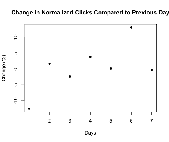
This showed that our metrics had significant variance day-over-day and explained why our exploitation points had such a different trend compared to exploration, which threw off the algorithm since our metric could be affected in similar ways by both click weight and time of day.

LinkedIn app usage varies significantly on each day of the week (e.g. professionals have different usage patterns on a Friday compared to a Wednesday), so seeing this sort of variance isn’t fully surprising.

This was particularly challenging since our tool expected data from exploration and exploitation to be on a similar trend; however, once we put exploration and exploitation data together (as required by the tool) the trend was lost. Because of these reasons, we decided to skip the exploitation phase to keep a reasonable trend under the time and ramp constraints we were working with.

 

Implementation of Online Autotuning: Revision of Optimization Problem

 
We then focused on applying the optimization problem on exploration data exclusively, which is shown below. We initially collected data at twice the online traffic requirement we set for ourselves at the beginning of the project (i.e requirement 2) to get a better understanding of our metrics. Figures 7a and 7b summarize the data collected The blue points in figure 7b correspond to the blue region in figure 7a, which is the feasible region as defined by our constraint.

 

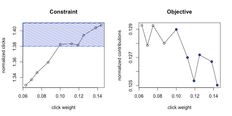
Our biggest challenge was figuring out how to deal with the noisiness of the contributions metrics. As we see from the plot of public contributions, even with twice the required ramp percentage, the contributions metric is very noisy. Given the limited traffic for our A/B experiments, we cannot trust the Contributions(????) metric.

In order to address this challenge, we took a closer look at the patterns of our metrics. Since the contributions metric is a decreasing function of ???? and our constraint is an increasing function of ????, the solution to the problem lies in the active set of constraints, normalizedClicks(????) = b. This is useful since normalizedClicks(????) is a much more stable metric. We could, therefore, reformulate our original problem as a minimization problem based on the original constraint, where we simply try to keep normalized clicks at the same level as the baseline, dropping our dependency on the normalizedContribuions metric:

 

 

The reformulated problem involves minimizing the normalizedClicksDelta with no constraints.

 

Implementation of Online AutoTuning: Final Strategy and Results

 
In figure 6a we observe our new metric over a range of click weights at 5% traffic for 2 days. Figure 6b shows the probability of click weight ???? (shown on the x-axis) being the optimal point in the optimization problem. This probability is calculated by first repeatedly sampling functions from the posterior Gaussian Process and then by identifying the point that optimizes (maximizes or minimizes) the sampled functions. The empirical distribution of the obtained points gives us figure 6b.

 

Previously, engineers would ramp multiple models with varying click weights in an attempt to find a properly tuned click weight model. This may involve relaunching different click weights a couple of days later if the first set of click weights did not contain an ideal click weight candidate. An example timeline of an actual model can involve 4 different click weights collected at 5% traffic for 2 days before selecting an “optimal” click weight. Figure 9 is an example of our ramping schedule before the introduction of click autotuning. Figure 10 is an example of the new ramping schedule with the autotuning tool

 

 

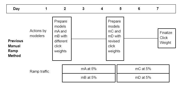
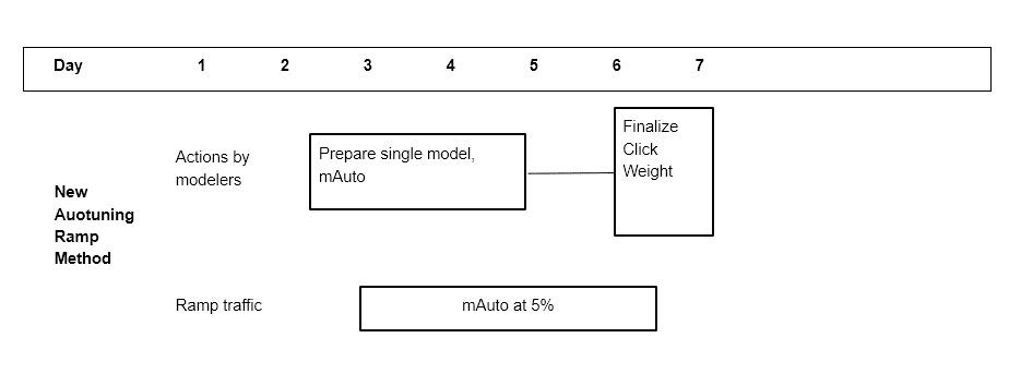
The old ramping schedule may take 10% traffic over 5 days (4 days to collect metrics and 1 day for the traffic change in between). Now with the automatic process of picking the parameter ????, we can reduce this part of the process to 2 days at 5% traffic. After a model ramps to 5%, the engineer can turn on click autotuning with a script and within 2 days we would be serving a single converged click weight. In these two days, we would be looking at 10 different click weights and choosing a solution that may lie between these points. This new tool improved our efficiency by reducing costs in the following three areas:

1. Ramp duration
2. Ramp volume
3. Manual efforts by engineers

In addition, the new tool also helped us find a more optimal click weight by being more precise in choosing ???? than previous manual efforts.

 

Lessons

 
We learned a few lessons along the way in this journey. First, we learned that in this particular optimization problem it pays to formulate your problem as simple as possible. After spending time to understand the metrics we wanted to target and how they related to our particular machine learning model, we realized we could switch our problem definition from a maximizing problem with constraints to just a minimization problem. This allowed us to work with just the constraint metric that was more reliable at lower ramp percentages, and it still allowed us to satisfy our general goal, which was to keep passive consumption constant between models while reducing both the manual effort required by engineers and online traffic requirements.

Also, it is important to be cognizant about the constraints that must be addressed for the solution to be practical. In our case, we could only allow the tool to use limited ramp volume and for a limited time to maximize the number of experiments, we can run at the same time. Once the constraints are well defined, it becomes more apparent which solutions are appropriate. In our case, the metrics we were working with had significant day-over-day, so we did not find explore-exploit algorithms helpful under our constraints since these algorithms required longer and bigger ramps for our problem space.

Thanks to Kinjal Basu, Viral Gupta, Yunbo Ouyang for building the parameter tuning library and all the advice, and our managers Ying Xuan and Zheng Li for their support.

 
Marco Varela is a Sr. Software Engineer at Linkedin, where he is a part of the Feed AI team and works on improving the ranking of updates on the Feed through a focus on automation and feature freshness.

Mavis Li is a software engineer on the Feed AI team at Linkedin working on personalization and ranking of the Feed. She has worked on various projects including adding downstream models as objectives, incorporating out of network group updates into the feed, and click weight autotuning.

Related:

• Check out this comprehensive guide to model optimization techniques.
• Automated Machine Learning: The Free eBook
• The Death of Data Scientists – will AutoML replace them?