Exploring the SwAV Method

This post discusses the SwAV (Swapping Assignments between multiple Views of the same image) method from the paper “Unsupervised Learning of Visual Features by Contrasting Cluster Assignments” by M. Caron et al.

comments

By Antonio Ferraioli, AI Aficionado

In this post we discuss SwAV (Swapping Assignments between multiple Views of the same image) method from the paper “Unsupervised Learning of Visual Features by Contrasting Cluster Assignments” by M. Caron et al.

For those interested in coding, several code repositories about SwAV algorithm are on GitHub; if in doubt, take a look at the repo mentioned in the paper.

Self-supervised learning of visual features

Supervised learning works with labeled training data; for example, in supervised image classification algorithms a cat photo needs to be annotated and labeled as “cat”. Self-supervised learning aims at obtaining features without using manual annotations. We will consider, in paticular, visual features.

There are two main classes of self-supervised learning methods for visual representation learning:

clustering-based methods require a pass over the entire dataset to form image “codes” (cluster assignments) that are used as targets during training, then some form of clustering is used to group similar image features;
contrastive methods use a loss function that explicitly compares pairs of image representations to push away representations from different images while pulling together those from transformations, or views, of the same image.

Online learning

Contrastive methods require computing all the pairwise comparisons on a large dataset; this is not practical. Typical clustering-based methods require to process entire datasets to determine codes, and this is expensive. A cheaper method would be better: online learning methods allow to train a system feeding a single data (or a mini-batch) instance at a time (no need to provide or process the whole input dataset at the start). The model can learn about new data on the fly and it keeps learning as new data comes in.

The SwAV method is a clustering-based online method whose goal is to learn visual features in an online fashion without supervision.

The method

The SwAV method computes a code from an augmented version of the image and predicts this code from other augmented versions of the same image.

Each image x_n (we suppose there are N original images in total) is transformed into an augmented view x_nt where t is a transformation like cropping, rotation, reducing image size, color change. The authors use a multi-crop stage where two standard resolution crops are used and V additional low resolution crops that cover only small parts of the image are sampled (V + 2 images in total, low resolution images ensures only a small increase in the compute cost).

The augmented view is mapped to a vector representation f_θ (x_nt) and this feature is then normalized into z_nt. In practice, f_θ is a sort of image encoder implemented by a convolutional neural network (ResNet50 for example) followed by a projection head that consists of a two layered MLP with ReLU activations.

After this normalization, a code q_nt is computed mapping z_nt to a set of K trainable normal vectors {c₁ , . . . , c_K}, called prototypes, that may be thought as the “clusters” in which the dataset should be partitioned (details about how to compute codes and update prototypes online are in the next paragraph). The number of prototypes K is given and not inferred. The authors set a default test value of 3000 prototypes for classification on ImageNet dataset. In neural networks implementation, a prototype vector is just the weights of a dense layer (with linear activation).

A little swapping trick comes in the end. Consider two different features z_t and z_s from two different augmentations of the same image and compute their codes q_t and q_s by matching these features to a set of K prototypes {c₁ , . . . , c_K}. Then consider the following loss:

L(z_t , z_s) = ℓ (z_t , q_s) + ℓ (z_s , q_t) .

The intuition is that if the two features z_t and z_s capture the same information (in essence, they are features deriving from the same image), then it should be possible to predict a given feature’s code from the other feature. The network and prototypes will be updated following this loss function.

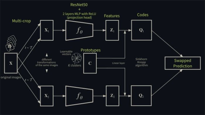Fig 1. SwAV architecture (enlarged)

Loss function details

The loss function has two terms. Each term represents the cross entropy loss between the code $\mathbf{q}_s^{(k)}$ and the probability $\mathbf{p}_t^{(k)}$ obtained by taking the softmax of the dot products of z_i and all prototypes, that is

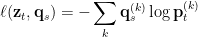
$\displaystyle \ell(\mathbf{z}_t, \mathbf{q}_s) = -\sum_k \mathbf{q}_s^{(k)} \log \mathbf{p}_t^{(k)}$

(k ranges over all prototypes) where for each fixed k

$\displaystyle \mathbf{p}_t^{(k)} = \frac{\exp(\frac{1}{\tau}\mathbf{z}_t^\top \mathbf{c}_k) }{\sum_{k'} \exp(\frac{1}{\tau}\mathbf{z}_t^\top \mathbf{c}_{k^{'}})} \,.$

The parameter τ is called temperature. The logarithm in the cross-entropy expression is applied element-wise. If we call C the matrix whose columns are the prototype vectors and if we use the fact that natural logarithm is the inverse function of exp, we can express the total loss for every image and for every pair of transformations varying in their respective domains:

$\displaystyle - \frac{1}{N}\sum_{n=1}^N \sum_{s,t\,\sim \mathcal{T}} \left[ \frac{1}{\tau} \mathbf{z}_{nt}^\top \mathbf{C} \mathbf{q}_{ns} + \frac{1}{\tau} \mathbf{z}_{ns}^\top \mathbf{C} \mathbf{q}_{nt} - \log \sum_{k=1}^K \exp \left( \frac{\mathbf{z}_{nt}^\top \mathbf{c}_k}{\tau} \right) - \log \sum_{k=1}^K \exp \left( \frac{\mathbf{z}_{ns}^\top \mathbf{c}_k}{\tau} \right) \right].$

Here C ≡ D ⨉ K, features z ≡ D ⨉ 1, codes q ≡ K ⨉ 1, prototypes c ≡ D ⨉ 1. The loss function is minimized jointly with respect to the prototypes C and the parameters θ of the image encoder f_θ. Prototype vectors are learned along with the ConvNet parameters by backpropragation.

Computing codes online

Codes are computed using only the image features within a batch to make the method online. A problem to solve is the cluster assignment: assign B samples [z₁ , . . . , z_B ] to K (prototype) clusters [ c₁ , . . . , c_K ].

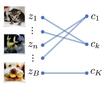Fig. 2. Cluster assignment

So we have to map B samples to K prototypes: let Q be the matrix representing this mapping. There is a trivial solution that must be discarded: assigning all samples to just one cluster! To solve this issue we introduce an equipartition constraint. Intuitively, we want that all prototypes are selected the same amounts of time. So, as a constraint, we restrict our attention only to those matrices whose projections onto their rows and columns — respectively — are probability distributions that split the data uniformly, which is captured by

r = 1/K · 1_K

c = 1/B · 1_B

where 1_K and 1_B are vectors of all ones of the appropriate dimensions. Therefore, we restrict our attention to the set

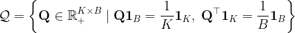$\displaystyle \mathcal{Q} = \left\{ \mathbf{Q} \in \mathbb{R}_{+}^{K \times B} \mid \mathbf{Q}\mathbf{1}_B = \frac{1}{K}\mathbf{1}_K, \; \mathbf{Q}^\top\mathbf{1}_K = \frac{1}{B}\mathbf{1}_B \right\}$ .

These constraints enforce that on average each prototype is selected at least B/K times in the batch.

We introduce a cost matrix, that is –C^⊤Z. Each entry of this matrix is the dot product between a sample and a prototype and roughly represents the cost we are going to pay when we assign a sample to a prototype.

	Cluster 1	Cluster 2	…	Cluster K
z₁	…	…	…	…
…	…	…	…	…
z_n	0.34	-0.83	…	0.92
…	…	…	…	…
z_B	…	…	…	…

We want to solve assignment problem under equipartition constraint and following a cost matrix.

Recall that, if M is a given D ⨉ D cost matrix, the cost of mapping r to c (two probability vectors) using a transport matrix (or joint probability) P can be quantified as ⟨P , M⟩, where ⟨.⟩ is the Frobenius product. If

$\mathbf{P} \in \left\{ \mathbf{A} \in \mathbb{R}_{+}^{D \times D} \mid \mathbf{A} \mathbf{1}_D = \mathbf{r}, \; \mathbf{A}^\top\mathbf{1}_D = \mathbf{c} \right\} \,,$

then the problem

$d_\mathbf{M}(\mathbf{r}, \mathbf{c}) := \min_\mathbf{\,P} \langle \mathbf{P}, \mathbf{M} \rangle$

is called optimal transport (OT) problem between r and c given cost M (Cuturi, 2013). In this setting it is easy to restate the cluster assignment as the optimal transport problem

$\underset{\mathbf{Q} \in \mathcal{Q}}{\min} \langle \mathbf{Q}, -\mathbf{C}^\top\mathbf{Z} \rangle + \varepsilon H(\mathbf{Q})$

where H is the entropy function

$\displaystyle H(\mathbf{Q}) = - \sum_{ij} \mathbf{Q}_{ij} \log \mathbf{Q}_{ij}$

and $\varepsilon$ is a parameter. In essence, $\varepsilon$ H(Q) is a regularization term. A solution to this regularized transport problem is in the form

$\displaystyle \mathbf{Q}^\ast = \mathrm{Diag}(\mathbf{u}) \exp\left(\frac{\mathbf{C}^\top\mathbf{Z}}{\varepsilon} \right) \mathrm{Diag}(\mathbf{v})$

where u ∈ ℝ^K and v ∈ ℝ^B are two non negative vectors and the center matrix is the element-wise exponential of the matrix C^⊤Z/ $\varepsilon$ . The vectors u and v are computed with a small number of matrix multiplications using the iterative Sinkhorn-Knopp algorithm (see next paragraph for pseudocode).

Pseudocode

The following PyTorch pseudocode provides a better overall understanding.

# C: prototypes (DxK)
# model: convnet + projection head
# temp: temperature

for x in loader: # load a batch x with B samples
    x_t = t(x) # t is a random augmentation
    x_s = s(x) # s is another random augmentation

    z = model(cat(x_t, x_s)) # embeddings: 2BxD

    scores = mm(z, C) # prototype scores: 2BxK
    scores_t = scores[:B]
    scores_s = scores[B:]

    # compute assignments
    with torch.no_grad():
        q_t = sinkhorn(scores_t)
        q_s = sinkhorn(scores_s)

    # convert scores to probabilities
    p_t = Softmax(scores_t / temp)
    p_s = Softmax(scores_s / temp)

    # swap prediction problem
    loss = - 0.5 * mean(q_t * log(p_s) + q_s * log(p_t))

    # SGD update: network and prototypes
    loss.backward()
    update(model.params)
    update(C)

    # normalize prototypes
    with torch.no_grad():
        C = normalize(C, dim=0, p=2)

The pseudocode for the Sinkhorn-Knopp algorithm is the following.

# Sinkhorn-Knopp
def sinkhorn(scores, eps=0.05, niters=3):
    Q = exp(scores / eps).T
    Q /= sum(Q)
    K, B = Q.shape
    u, r, c = zeros(K), ones(K) / K, ones(B) / B
    for _ in range(niters):
        u = sum(Q, dim=1)
        Q *= (r / u).unsqueeze(1)
        Q *= (c / sum(Q, dim=0)).unsqueeze(0)
    return (Q / sum(Q, dim=0, keepdim=True)).T

Check the original article code implementation using PyTorch here.

Useful links

Original SwAV paper.

Original code implementation here.

Paper about optimal transport here.

Interesting video on the SwAV method.

Bio: Antonio Ferraioli is an AI aficionado living in southern Italy. Admin of "m0nads", a blog about AI (and its subfields) and Data Science.

Original. Reposted with permission.

Related: