Comparing Machine Learning Models: Statistical vs. Practical Significance
Is model A or B more accurate? Hmm… In this blog post, I’d love to share my recent findings on model comparison.
By Dina Jankovic, Hubdoc

Left or right?
A very shallow approach would be to compare the overall accuracy on the test set, say, model A’s accuracy is 94% vs. model B’s accuracy is 95%, and blindly conclude that B won the race. In fact, there is so much more than the overall accuracy to investigate and more facts to consider.
In this blog post, I’d love to share my recent findings on model comparison. I like using simple language when explaining statistics, so this post is a good read for those who are not so strong in statistics, but would love to learn a little more.
1. “Understand” the Data
If possible, it’s a really good idea to come up with some plots that can tell you right away what’s actually going on. It seems odd to do any plotting at this point, but plots can provide you with some insights that numbers just can’t.
In one of my projects, my goal was to compare the accuracy of 2 ML models on the same test set when predicting user’s tax on their documents, so I thought it’d be a good idea to aggregate the data by user’s id and compute the proportion of correctly predicted taxes for each model.
The data set I had was big (100K+ instances), so I broke down the analysis by region and focused on smaller subsets of data — the accuracy may differ from subset to subset. This is generally a good idea when dealing with ridiculously large data sets, simply because it is impossible to digest a huge amount of data at once, let alone come up with reliable conclusions (more about the sample size issue later). A huge advantage of a Big Data set is that not only you have an insane amount of information available, but you can also zoom in the data and explore what’s going on on a certain subset of pixels.
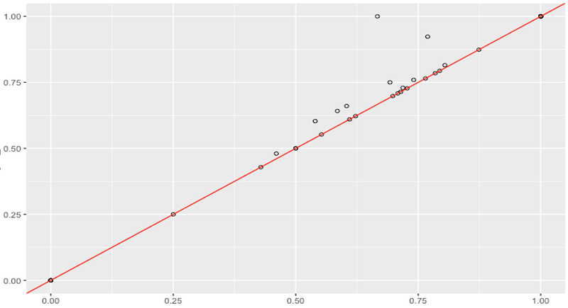
subset 1: model A vs. model B scores
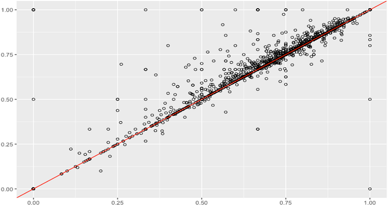
subset 2: model A vs. model B scores

subset 2: model A is clearly doing better than B… look at all those spikes!
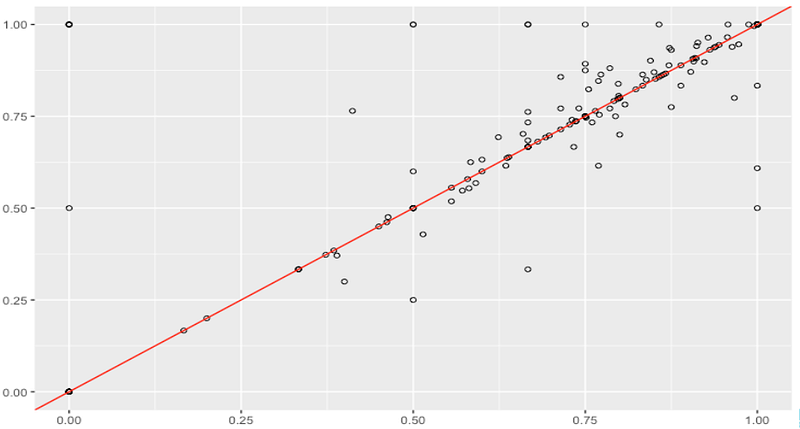
subset 3: model A vs. model B scores
2. Hypothesis Testing: Let’s do it right!
It seems trivial at the first sight, and you’ve probably seen this before:
- Set up H0 and H1
- Come up with a test-statistic, and assume Normal distribution out of the blue
- Somehow calculate the p-value
- If p < alpha = 0.05 reject H0, and ta-dam you’re all done!
In practice, hypothesis testing is a little more complicated and sensitive. Sadly, people use it without much caution and misinterpret the results. Let’s do it together step by step!
Step 1. We set up H0: the null hypothesis = no statistically significant difference between the 2 models and H1: the alternative hypothesis = there is a statistically significant difference between the accuracy of the 2 models — up to you: model A != B (two-tailed) or model A < or > model B (one-tailed)
Step 2. We come up with a test-statistic in such a way as to quantify, within the observed data, behaviours that would distinguish the null from the alternative hypothesis. There are many options, and even the best statisticians could be clueless about an X number of statistical tests — and that’s totally fine! There are way too many assumptions and facts to consider, so once you know your data, you can pick the right one. The point is to understand how hypothesis testing works, and the actual test-statistic is just a tool that is easy to calculate with a software.
Beware that there is a bunch of assumptions that need to be met before applying any statistical test. For each test, you can look up the required assumptions; however, the vast majority of real life data is not going to strictly meet all conditions, so feel free to relax them a little bit! But what if your data, for example, seriously deviates from Normal distribution?
There are 2 big families of statistical tests: parametric and non-parametrictests, and I highly recommend reading a little more about them here. I’ll keep it short: the major difference between the two is the fact that parametric tests require certain assumptions about the population distribution, while non-parametric tests are a bit more robust (no parameters, please!).
In my analysis, I initially wanted to use the paired samples t-test, but my data was clearly not normally distributed, so I went for the Wilcoxon signed rank test (non-parametric equivalent of the paired samples t-test). It’s up to you to decide which test-statistic you’re going to use in your analysis, but always make sure the assumptions are met.
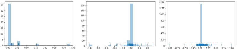
My data wasn’t normally distributed :(
Luckily, the p-value can be easily found in R/Python so you don’t need to torture yourself and do it manually, and although I’ve been mostly using Python, I prefer doing hypothesis testing in R since there are more options available. Below is a code snippet. We see that on subset 2, we indeed obtained a small p-value, but the confidence interval is useless.
> wilcox.test(data1, data2, conf.int = TRUE, alternative="greater", paired=TRUE, conf.level = .95, exact = FALSE)

V = 1061.5, p-value = 0.008576
alternative hypothesis: true location shift is less than 0
95 percent confidence interval:
-Inf -0.008297017
sample estimates:
(pseudo)median
-0.02717335
Step 4. Very straightforward: if p-value < pre-specified alpha (0.05, traditionally), you can reject H0 in favour of H1. Otherwise, there is not enough evidence to reject H0, which does not mean that H0 is true! In fact, it may still be false, but there was simply not enough evidence to reject it, based on the data. If alpha is 0.05 = 5%, that means there is only a 5% risk of concluding a difference exists when it actually doesn’t (aka type 1 error). You may be asking yourself: so why can’t we go for alpha = 1% instead of 5%? It’s because the analysis is going to be more conservative, so it is going to be harder to reject H0 (and we’re aiming to reject it).
The most commonly used alphas are 5%, 10% and 1%, but you can pick any alpha you’d like! It really depends on how much risk you’re willing to take.
Can alpha be 0% (i.e. no chance of type 1 error)? Nope :) In reality, there’s always a chance you’ll commit an error, so it doesn’t really make sense to pick 0%. It’s always good to leave some room for errors.
If you wanna play around and p-hack, you may increase your alpha and reject H0, but then you have to settle for a lower level of confidence (as alpha increases, confidence level goes down — you can’t have it all :) ).
3. Post-hoc Analysis: Statistical vs. Practical Significance
If you get a ridiculously small p-value, that certainly means that there is astatistically significant difference between the accuracy of the 2 models. Previously, I indeed got a small p-value, so mathematically speaking, the models differ for sure, but being “significant” does not imply being important. Does that difference actually mean anything? Is that small difference relevant to the business problem?
Statistical significance refers to the unlikelihood that mean differences observed in the sample have occurred due to sampling error. Given a large enough sample, despite seemingly insignificant population differences, one might still find statistical significance. On the other side, practical significance looks at whether the difference is large enough to be of value in a practical sense. While statistical significance is strictly defined, practical significance is more intuitive and subjective.

At this point, you may have realized that p-values are not super powerful as you may think. There’s more to investigate. It’d be great to consider the effect size as well. The effect size measures the magnitude of the difference — if there is a statistically significant difference, we may be interested in its magnitude. Effect size emphasizes the size of the difference rather than confounding it with sample size.
> abs(qnorm(p-value))/sqrt(n)

0.14

# the effect size is small
What is considered a small, medium, large effect size? The traditional cut-offs are 0.1, 0.3, 0.5 respectively, but again, this really depends on your business problem.
And what’s the issue with the sample size? Well, if your sample is too small, then your results are not going to be reliable, but that’s trivial. What if your sample size is too large? This seems awesome — but in that case even the ridiculously small differences could be detected with a hypothesis test. There’s so much data that even the tiny deviations could be perceived as significant. That’s why the effect size becomes useful.
There’s more to do — we could try to find the power or the test and the optimal sample size. But we’re good for now.
Hypothesis testing could be really useful in model comparison if it’s done right. Setting up H0 & H1, calculating the test-statistic and finding the p-value is routine work, but interpreting the results require some intuition, creativity and deeper understanding of the business problem. Remember that if the testing is based on a very large test set, relationships found to be statistically significant may not have much practical significance. Don’t just blindly trust those magical p-values: zooming in the data and conducting a post-hoc analysis is always a good idea! :)
Feel free to reach out to me via email or LinkedIn, I’m always up for a chat about Data Science!
Bio: Dina Jankovic is a Data Analyst in the Data Science team at Hubdoc in Toronto, Canada. She earned her BSc in Math from University of Belgrade and MSc in Statistics from University of Ottawa. She utilizes computational statistics and machine learning techniques to make smart business decisions and better understand the world.
Original. Reposted with permission.
Related: