 Explore the world of Bioinformatics with Machine Learning
 Explore the world of Bioinformatics with Machine Learning
The article contains a brief introduction of Bioinformatics and how a machine learning classification algorithm can be used to classify the type of cancer in each patient by their gene expressions.
Bioinformatics is a field of study that uses computation to extract knowledge from biological data. It includes the collection, storage, retrieval, manipulation and modeling of data for analysis, visualization or prediction through the development of algorithms and software.
We can quote it in a simpler way “Bioinformatics deals with computational and mathematical approaches for understanding and processing biological data”.
It is an interdisciplinary field in which new computational methods are developed to analyze biological data and to make biological discoveries. For example, two typical tasks in genetics and genomics are the processes of sequencing and annotating an organism’s complete set of DNA. In neurosciences, neuroimaging techniques, such as computerized tomography (CT), positron emission tomography (PET), functional magnetic resonance imaging (fMRI), and diffusion tensor imaging (DTI), are used to study brains in vivo and to understand the inner workings of the nervous system.
The application of Machine Learning to biological and neuroimaging data opens new frontiers for biomedical engineering: improving our understanding of complex diseases such as cancer or neurodegenerative and psychiatric disorders. Advances in this field can ultimately lead to the development of automated diagnostic tools and of precision medicine, which consists of targeting custom medical treatments considering individual variability, lifestyle, and environment.
Prior to the emergence of machine learning algorithms, bioinformatics algorithms had to be explicitly programmed by hand which, for problems such as protein structure prediction, proves extremely difficult.
Machine learning techniques such as deep learning enable the algorithm to make use of automatic feature learning which means that based on the dataset alone, the algorithm can learn how to combine multiple features of the input data into a more abstract set of features from which to conduct further learning. This multi-layered approach to learning patterns in the input data allows such systems to make quite complex predictions when trained on large datasets. In recent years, the size and number of available biological datasets have skyrocketed, enabling bioinformatics researchers to make use of these machine learning algorithms.
Machine learning has been applied to six biological domains: Genomics, Proteomics, Microarrays, Systems biology, Stroke diagnosis, and Text mining.
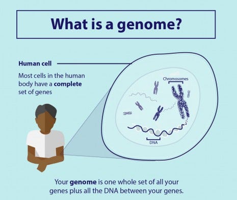
Genomics
It is an interdisciplinary field of biology focusing on the structure, function, evolution, mapping, and editing of genomes. A Genome is an organism’s complete set of DNA, including all of its genes. There is an increasing need for the development of machine learning systems that can automatically determine the location of protein-encoding genes within a given DNA sequence and this problem in computational biology is known as gene prediction. To know more about Genomics click here.
Proteomics
Proteomics is the large-scale study of proteomes. A proteome is a set of proteins produced in an organism, system, or biological context.

Proteins, strings of amino acids, gain much of their function from protein folding in which they conform into a three-dimensional structure. This structure is composed of a number of layers of folding, including the primary structure (i.e. the flat string of amino acids), the secondary structure (alpha helices and beta sheets), the tertiary structure, and the quarternary structure.
Protein secondary structure prediction is the main focus of this subfield as the further protein foldings (tertiary and quaternary structures) are determined based on the secondary structure. Solving the true structure of a protein is an incredibly expensive and time-intensive process, furthering the need for systems that can accurately predict the structure of a protein by analyzing the amino acid sequence directly. Prior to machine learning, researchers needed to conduct this prediction manually.
The current state-of-the-art in secondary structure prediction uses a system called DeepCNF (deep convolutional neural fields) which relies on the machine learning model of artificial neural networks to achieve an accuracy of approximately 84% when tasked to classify the amino acids of a protein sequence into one of three structural classes (helix, sheet, or coil).
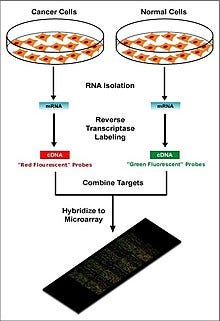
Microarrays
Microarrays, a type of lab-on-a-chip, are used for automatically collecting data about large amounts of biological material. Machine learning can aid in the analysis of this data, and it has been applied to expression pattern identification, classification, and genetic network induction.
This technology is especially useful for monitoring the expression of genes within a genome, aiding in diagnosing different types of cancer-based on which genes are expressed. One of the main problems in this field is identifying which genes are expressed based on the collected data.
Machine learning presents a potential solution to this problem as various classification methods can be used to perform this identification. The most commonly used methods are radial basis function networks, deep learning, Bayesian classification, decision trees, and random forest.
Systems biology
Systems biology focuses on the study of the emergent behaviors from complex interactions of simple biological components in a system. Such components can include molecules such as DNA, RNA, proteins, and metabolites.
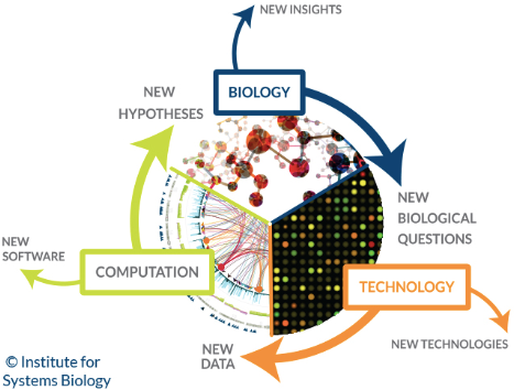
Machine learning has been used to aid in the modeling of these complex interactions in biological systems in domains such as genetic networks, signal transduction networks, and metabolic pathways. Probabilistic graphical models, a machine learning technique for determining the structure between different variables, are one of the most commonly used methods for modeling genetic networks. In addition, machine learning has been applied to systems biology problems such as identifying transcription factor binding sites using a technique known as Markov chain optimization. Genetic algorithms, machine learning techniques which are based on the natural process of evolution, have been used to model genetic networks and regulatory structures.
Stroke diagnosis
Machine learning methods for the analysis of neuroimaging data are used to help diagnose stroke. Three-dimensional Convolutional Neural Network(CNN) and Support Vector Machines(SVM) methods are often used.
Text mining
The increase in available biological publications led to the issue of the increase in difficulty in searching through and compiling all the relevant available information on a given topic across all sources. This task is known as knowledge extraction. This is necessary for biological data collection which can then, in turn, be fed into machine learning algorithms to generate new biological knowledge. Machine learning can be used for this knowledge extraction task using techniques such as Natural Language Processing(NLP) to extract useful information from human-generated reports in a database.
This technique has been applied to the search for novel drug targets, as this task requires the examination of information stored in biological databases and journals. Annotations of proteins in protein databases often do not reflect the complete known set of knowledge of each protein, so additional information must be extracted from biomedical literature. Machine learning has been applied to the automatic annotation of the function of genes and proteins, determination of the subcellular localization of a protein, analysis of DNA-expression arrays, large-scale protein interaction analysis, and molecule interaction analysis.
Lets us now implement the Support Vector Machine(SVM) algorithm in bioinformatics dataset and see how it works.
Molecular Classification of Cancer by Gene Expression Monitoring using Support Vector Machine(SVM)
Although cancer classification has improved over the past 30 years, there has been no general approach for identifying new cancer classes (class discovery) or for assigning tumors to known classes (class prediction). The dataset comes from a proof-of-concept study published in 1999 by Golub et al. It showed how new cases of cancer could be classified by gene expression monitoring (via DNA microarray) and thereby provided a general approach for identifying new cancer classes and assigning tumors to known classes.
The goal is to classify patients with acute myeloid leukemia (AML) and acute lymphoblastic leukemia (ALL) using the SVM algorithm.
The dataset can be downloaded from Kaggle.
Let's start coding:
Start with loading 3 basic python libraries:
import pandas as pd
import numpy as np
import matplotlib.pyplot as plt
Load the datasets:
Train_Data = pd.read_csv("/.../bioinformatics/data_set_ALL_AML_train.csv")
Test_Data = pd.read_csv("/.../bioinformatics/data_set_ALL_AML_independent.csv")
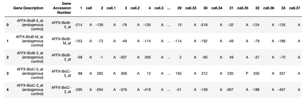
labels = pd.read_csv("/.../bioinformatics/actual.csv", index_col = 'patient')Train_Data.head()
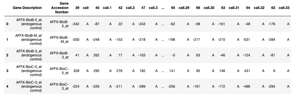
Test_Data.head()
About the dataset:
- Each row represents a different gene.
- Columns 1 and 2 are descriptions about that gene.
- Each numbered column is a patient in label data.
- Each patient has 7129 gene expression values — i.e each patient has one value for each gene.
- The training data contain gene expression values for patients 1 through 38.
- The test data contain gene expression values for patients 39 through 72
Now check for nulls in both the datasets(We don't have any nulls in these datasets).
print(Train_Data.isna().sum().max())
print(Test_Data.isna().sum().max())
Now drop column ‘call’ from both train and test data as it doesn't have any statistical relevance.
cols = [col for col in Test_Data.columns if 'call' in col]
test = Test_Data.drop(cols, 1)
cols = [col for col in Train_Data.columns if 'call' in col]
train = Train_Data.drop(cols, 1)
Now join all the datasets and transpose the final joined data.
patients = [str(i) for i in range(1, 73, 1)]
df_all = pd.concat([train, test], axis = 1)[patients]
df_all = df_All.T
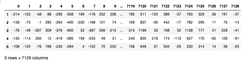
After transpose, the rows have been converted to columns(7129 columns/features)
Now convert patient column to a numeric value and create dummy variables(converts categories into numeric values) since ‘cancer’ is a cateogorical column having 2 categories(ALL, AML).
df_all["patient"] = pd.to_numeric(patients)
labels["cancer"]= pd.get_dummies(Actual.cancer, drop_first=True)
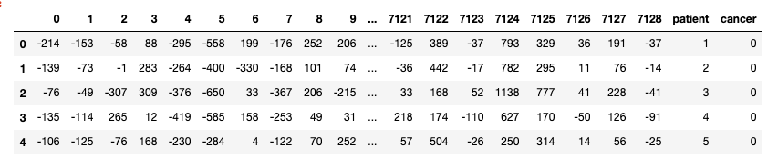
Now join data frames df_all and labels on patient column.
Data = pd.merge(df_all, labels, on="patient")
Data.head()
Our next step is to create two variables X(matrix of independent variables) and y(vector of the dependent variable).
X, y = Data.drop(columns=["cancer"]), Data["cancer"]
Next, We split 75% of the data into training set while 25% of the data to test set. The test_size variable is where we actually specify the proportion of the test set.
from sklearn.model_selection import train_test_split
X_train, X_test, y_train, y_test =  train_test_split(X,y,test_size = 0.25, random_state= 0)
Next step is to normalize the data because if we closely look at the data the range of values of independent variables varies a lot. So when the values vary a lot in independent variables, we use feature scaling so that all the values remain in the comparable range.
from sklearn.preprocessing import StandardScaler
sc_X = StandardScaler()
X_train = sc_X.fit_transform(X_train)
X_test = sc_X.transform(X_test)
The number of columns/features that we have been working with is huge. We have 72 rows and 7129 columns. Basically we need to decrease the number of features(Dimentioanlity Reduction) to remove the possibility of Curse of Dimensionality.
For reducing the number of dimensions/features we will use the most popular dimensionality reduction algorithm i.e. PCA(Principal Component Analysis).
To perform PCA we have to choose the number of features/dimensions that we want in our data.
from sklearn.decomposition import PCA
pca = PCA()
X_train = pca.fit_transform(X_train)
X_test = pca.transform(X_test)
total=sum(pca.explained_variance_)
k=0
current_variance=0
while current_variance/total < 0.90:
    current_variance += pca.explained_variance_[k]
    k=k+1
The above code gives k=38.
Now let us take k=38 and apply PCA on our independent variables.
from sklearn.decomposition import PCA
pca = PCA(n_components = 38)
X_train = pca.fit_transform(X_train)
X_test = pca.transform(X_test)cum_sum = pca.explained_variance_ratio_.cumsum()
cum_sum = cum_sum*100
plt.bar(range(38), cum_sum)
plt.ylabel("Cumulative Explained Variance")
plt.xlabel("Principal Components")
plt.title("Around 90% of variance is explained by the First 38 columns ")
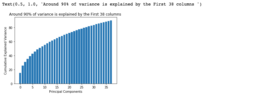
Note:- PCA can lead to a reduction in model performance on datasets with no or low feature correlation or does not meet the assumptions of linearity.
The next step is to fit our data into the Support Vector Machine(SVM) algorithm but before doing that we will perform Hyperparameter optimization.
Hyperparameter optimization or tuning is the problem of choosing a set of optimal hyperparameters for a learning algorithm. A hyperparameter is a parameter whose value is used to control the learning process. By contrast, the values of other parameters are learned.
We will use GridSearchCV from sklearn for choosing the best hyperparameters.
from sklearn.model_selection import GridSearchCV
from sklearn.svm import SVCparameters = [{'C': [1, 10, 100, 1000], 'kernel': ['linear']},
              {'C': [1, 10, 100, 1000], 'kernel': ['rbf'], 'gamma': [0.1, 0.2, 0.3, 0.4, 0.5, 0.6, 0.7, 0.8, 0.9]}]search = GridSearchCV(SVC(), parameters, n_jobs=-1, verbose=1)
search.fit(X_train, y_train)
Now check what are the best parameters for our SVM algorithm
best_parameters = search.best_estimator_

Now let's train our SVM classification model.
model = SVC(C=1, cache_size=200, class_weight=None, coef0=0.0,
    decision_function_shape='ovr', degree=3, gamma='auto_deprecated',
    kernel='linear', max_iter=-1, probability=False, random_state=None,
    shrinking=True, tol=0.001, verbose=False)

model.fit(X_train, y_train)
Its time for some predictions:
y_pred=model.predict(X_test)
Evaluating model performance:
from sklearn.metrics import accuracy_score, confusion_matrixfrom sklearn import metrics
print('Accuracy Score:',round(accuracy_score(y_test, y_pred),2))
#confusion matrix
cm = confusion_matrix(y_test, y_pred)Output:
Accuracy Score: 0.67
Confusion matrix and visualize it using Heatmap.
class_names=[1,2,3]
fig, ax = plt.subplots()from sklearn.metrics import confusion_matrix
import seaborn as snscm = confusion_matrix(y_test, y_pred)class_names=['ALL', 'AML']
fig, ax = plt.subplots()
tick_marks = np.arange(len(class_names))
plt.xticks(tick_marks, class_names)
plt.yticks(tick_marks, class_names)
sns.heatmap(pd.DataFrame(cm), annot=True, cmap="viridis" ,fmt='g')
ax.xaxis.set_label_position("top")
plt.tight_layout()
plt.title('Confusion matrix', y=1.1)
plt.ylabel('Actual label')
plt.xlabel('Predicted label')
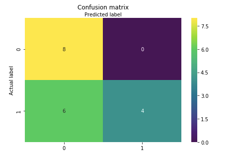
Well, this example goes to show that if you just predict that every patient has AML, you’ll be correct more often than wrong.
So our SVM classification model predicted the cancer patients with 67% accuracy which is of course not that good. What you can do is try different classifiers like Random forest, K-NN, Gradient Boosting, xgboost etc and compare the accuracies for each model.
Conclusion
So in this article, we have seen how a classification ML algorithm can be used to predict cancer in a patient.
Ultimately I think for machine learning to really flourish, it's going to come down to better bioinformatics data. Heath and bioinformatics data right now have pretty poor statistical power. Either they usually have poor signal (genomics), high noise/bias (electronic health records), or smallish sample sizes.
Well, that is all for this article. I hope you guys have enjoyed reading it, please share your suggestions/views/questions in the comment section.
You can also reach me out over LinkedIn for any query.

Thanks for reading !!!
Bio: Nagesh Singh Chauhan is a Data Science enthusiast. Interested in Big Data, Python, Machine Learning.
Original. Reposted with permission.
Related:
- A Friendly Introduction to Support Vector Machines
- Classifying Heart Disease Using K-Nearest Neighbors
- Introduction to Image Segmentation with K-Means clustering