Overview of data distributions

By Madalina Ciortan, Data scientist, PhD researcher in bioinformatics at ULB.

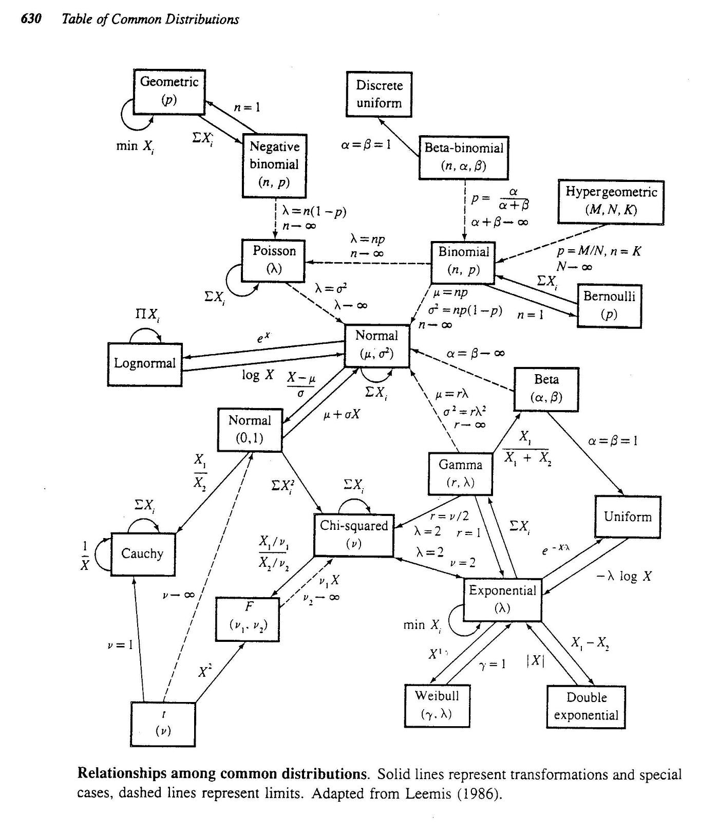
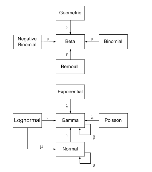
There are over 20 different types of data distributions (applied to the continuous or the discrete space) commonly used in data science to model various types of phenomena. They also have many interconnections, which allow us to group them in a family of distributions. A great blog post proposes the following visualization, where the continuous lines represent an exact relationship (special case, transformation or sum), and the dashed line indicates a limit relationship. The same post provides a detailed explanation of these relationships, and this paper provides a thorough analysis of the interactions between distributions.

The following section provides information about each type of distribution depicting what phenomena it typically models, some example scenarios illustrating when it makes sense to choose the distribution, the probability distribution/mass function, and its typical shape in a visualization.

The probability density function is a continuous approximation in terms of integrals of the density of a distribution or a smooth version of histograms. Cumulative distribution function can be expressed as F(x)= P(X ≤x), indicating the probability of X taking on a less than or equal value to x. PMF functions apply to the discrete domain and give the probability that a discrete random variable is exactly equal to some value.

 

Discrete distributions

 

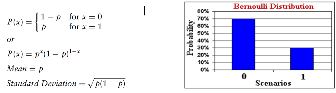
Bernoulli distribution is a discrete distribution consisting of only one trial with 2 outcomes (success/failure). It constitutes the basis for defining other more complex distributions, which analyze more than one trial, such as the next 3 distributions.

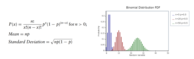
Binomial distribution computes the probability of k successes within n trials. Like the Bernoulli distribution, trials are independent and have 2 outcomes. Examples of using this distribution are for estimating the number of heads given a series of n coin tosses or how many winning lottery tickets we can expect given the total number of tickets bought. This distribution has 2 parameters, n the total number of trials and p the probability of success:

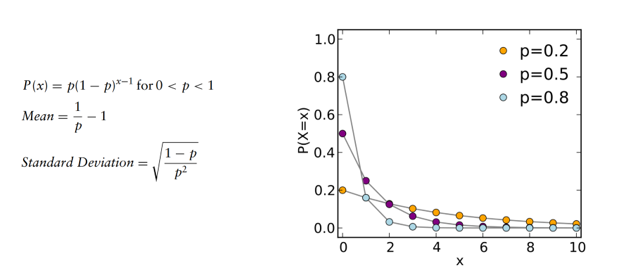
Geometric distribution computes the number of trials before the first success occurs. The number of trials is not fixed, so the probability of success is the same throughout the independent trials, and the experiment continues until the first success. This distribution has one parameter, the probability of success p.

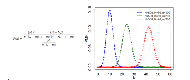
Hypergeometric distribution measures the number of successes in n trial (similar to binomial) but it doesn’t rely on an assumption of independence between trials. Thus, the trials are performed without replacement, and each trial changes the probability of success. Examples are the probability of drawing a certain combination of cards from a deck without replacement or selecting defective light bulbs from a crate having both defective and working light bulbs. This distribution depends on the number of items in the population (N), the number of trials sampled (n), and the number of items in the population having the successful trait Nx. x represents the number of successful trials.

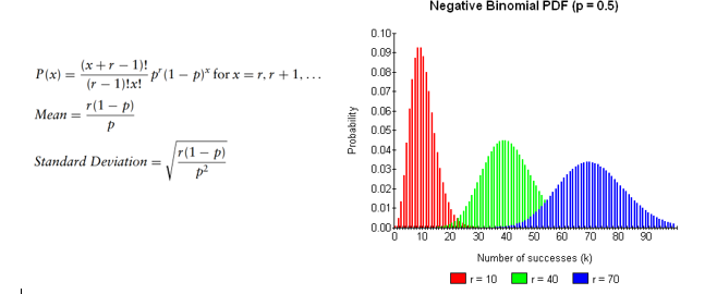
Negative binomial computes the number of trials until reaching r successful events. It is a superdistribution of the geometric distribution and can be used to model situations like the number of sales calls to be performed in order to close r deals. The parameters used by this distribution are the probability of success p and the number of required successes r.

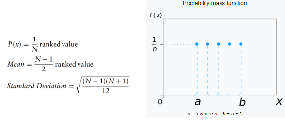
Discrete uniform is the distribution of n different but equally likely outcomes. It is the counterpart of uniform distribution in the discrete space. It takes as input only N, the number of distinct outcomes.

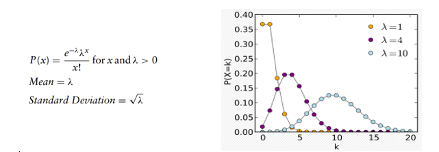
Poisson distribution approximates the number of times an event occurs in a given interval, knowing that the occurrences are independent, there is no upper limit to the the number of events and the average number of occurrences must remain the same if we extended the analysis form one interval to another. This distribution has one parameter, lambda, being the average number of events per interval.

 

Continuous distributions

 

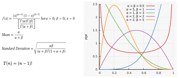
Beta distribution is commonly used to represent variability over a fixed range. For instance, to model the behavior of random variables limited to intervals of finite length. It is also a suitable choice to model percentage or proportions. In Bayesian inference, it is used to model the conjugate prior for Bernoulli, Binomial, Negative binomial and geometric distributions. More simply put, the beta distribution is a good proposal for the priors (the initial knowledge of success) for different applications from the Bernoulli family, such as the number of heads on coin tossing trials or any other dual outcome event. It takes 2 parameters, alpha and beta, and the uncertain variable is a random value between 0 and a positive value. Different combinations of alpha and beta lead to the following shapes of the distribution:

• alpha == beta => symmetrical distribution
• if (alpha == 1 and beta > 1) or (beta== 1 and alpha> 1) => J shaped distribution
• alpha < beta => positive skew
• alpha >beta => negative skew

Dirichlet distribution is a multivariate generalization of beta distributions, for which reason it is also known as Multivariate Beta distributions. It is used as prior distribution in Bayesian statistics, where it is the conjugate prior of the categorical and multinomial distribution. It is parameterized by a vector alpha of positive reals, and it samples over a probability simplex. A probability simplex is a set of k numbers adding up to 1 and which correspond to the probabilities of k classes. A k-dimensional Dirichlet distribution has k parameters.

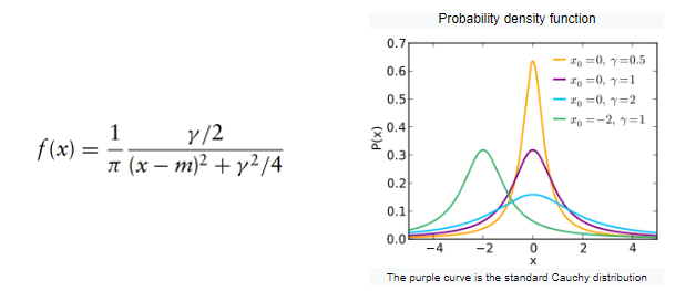
Cauchy distribution is employed in mechanical and electrical theory, physical anthropology and measurement, and calibration problems. In physics, it describes the distribution of the energy of an unstable state in quantum mechanics under the name Lorentzian distribution. Another application is to model the points of impact of a fixed straight line of particles emitted from a point source or in robustness studies. The Cauchy distribution is known to be a pathological distribution as both its mean and variance are undefined. It takes two parameters. In Bayesian statistics, Cauchy distribution can be used to model the priors for the regression coefficients in logistic regression.

The distribution takes two parameters, the mode m (corresponding to the peak) and the scale gamma (half-width at half maximum of the distribution). Cauchy distribution is the Student’s T distribution with 1 degree of freedom.

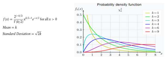
Chi-Square distribution is predominantly used in hypothesis testing, in the construction of confidence intervals, in the evaluation of the goodness of fit of an observed distribution to a theoretical one. Chi-Square (with one degree of freedom) variable is the square of a standard normal variable, and Chi-Square distribution has additive property (Sum of two independent Chi-Square distributions is also a Chi-Square variable). The sum of k independent normal distributions is distributed as a chi-square with k degrees of freedom. The chi-square distribution can also be modeled using a gamma distribution with the shape parameter as k/2 and scale as 2S².

The chi-squared distribution has one parameter: k, the number of degrees of freedom.

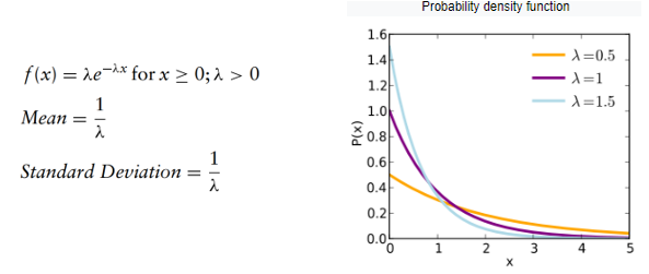
Exponential distribution describes the amount of time between events occurring at random moments. It is considered that time has no effect on future outcomes (the future lifetime of an object has the same distribution, regardless of the time it existed) which makes the exponential “memoryless”. It can be used to model situations such as: how long do we have to wait at a crossroads until we see a car running on the red light or how long it will take until someone receives the next phone call? How long will a product function before breaking down?

The exponential distribution is related to Poisson, which doesn’t describe the time lapsed but the number of occurrences of an event in a given time frame. The exponential distribution is parametrized only by lambda, the success rate.

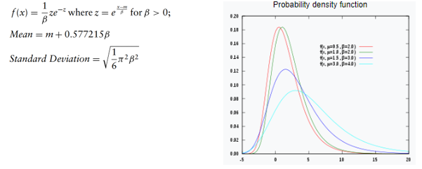
Extreme value distribution, or the Gumbel distribution, models the distribution of the maximum (or the minimum) of a number of samples of various distributions. Examples of this distribution are the breaking strengths of materials, the maximum load for an aircraft, tolerance studies, the maximum level of a river, or of an earthquake in a given year. This distribution has 2 parameters, the mode m corresponding to the most likely point (or the PDF’s highest peak) and a scale parameter, beta, which is > 0 and governs the variance.

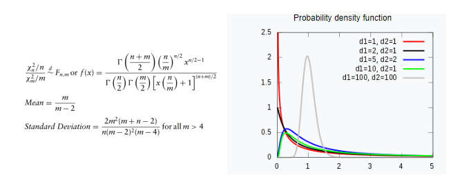
F distribution is used to test the statistical difference between two variances as part of one way ANOVA analysis or the overall significance of a regression model with f-tests. Frequently it is the null distribution (the probability distribution when the null hypothesis is true) of test statistics. It takes as parameters n degrees of freedom for the numerator and m degrees of freedom for the denominator.

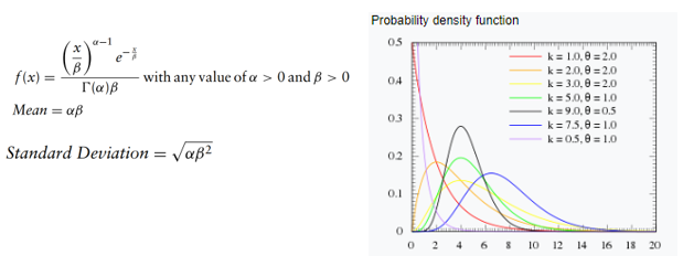
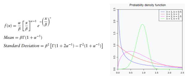
Gamma distribution is used to measure the time between the occurrence of events when the event process is not completely random. The number of events in the studied time frame is not limited to a fixed number. The events are independent. Gamma distribution is related to lognormal, exponential Pascal, Poisson, and chi-square distributions. It can be used to model pollutant concentrations and precipitation quantities in meteorological processes. It depends on 2 parameters, alpha or the shape parameter and beta, the scale parameter.

A special case arises when alpha is a positive integer, in which case the distribution (also known as the Erlang distribution) can be used to predict waiting times in queuing systems.

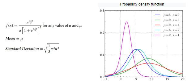
Logistic distribution is used to describe population growth over time or chemical reactions. This distribution is symmetrical and takes 2 parameters: the mean or the average value and the scale, controlling the variance.

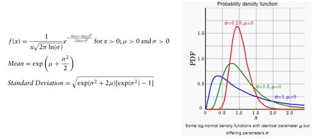
Lognormal distribution is a good candidate for modelling positively skewed values, which are ≥ 0. For instance, the normal distribution cannot be used to model stock prices because it has a negative side, and stock prices cannot fall below zero, so lognormal distribution is a good candidate. Thus, if a random variable X is log-normally distributed, then Y = ln(X) has a normal distribution. Likewise, if Y has a normal distribution, then the exponential function of Y, X = exp(Y), has a lognormal distribution. The lognormal distribution is described by 2 parameters, the mean and the standard deviation.

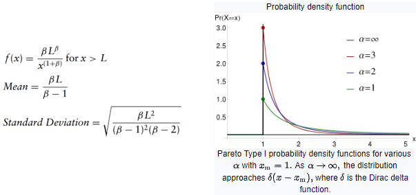
Pareto distribution is a power-law probability distribution used to model empiric phenomena such as the distribution of wealth, the stock price fluctuations, the occurrence of natural resources. Pareto distribution has been vulgarized under the name of Pareto principle (or the “80–20 rule”, the Matthew principle) stating that, for example, 80% of the wealth of a society is held by 20% of its population. However, the Pareto distribution only produces this result for a particular power value of the input parameter alpha (α = log45 ≈ 1.16). In terms of parameters, this distribution depends on the location (the lower bound for the variable) and the shape controlling the variance.

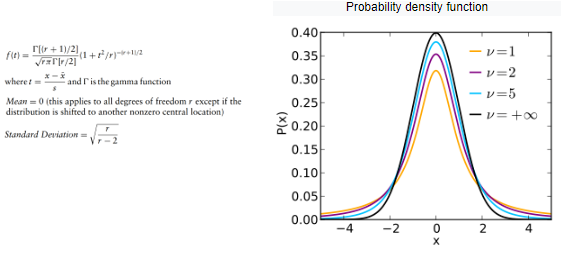
Student’s t distribution is typically used to test the statistical significance of the difference between two sample means or to estimate the mean of a normally distributed population, both for small sample sizes. The shape of this distribution resembles the bell shape of a leptokurtic gaussian. The only parameter is the degree of freedom r.

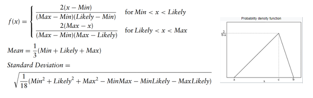
Triangular distribution describes the situation where the minimum, maximum, and most likely values of an event are known. Both the minimum and the maximum values are fixed, and the most likely value falls between them, forming a triangular-shaped distribution. For instance, this distribution can describe the sales of a product when we know the minimum, maximum, and most likely estimations.

Weibull distribution is heavily employed in fatigue tests, e.g., to describe failure time in reliability studies or breaking strengths of materials in quality control tests. It can also be used to model physical quantities, such as wind speed. It depends on 3 input parameters: the location L, the shape alpha, and the scale beta. When the shape parameter = 1, it becomes the exponential distribution.

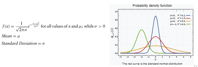
Normal distribution is probably the most studied distribution, and is used to describe natural phenomena, such as the distribution of heights and IQ scores. This distribution takes as input 2 parameters, the mean and the standard deviation.

Conjugate distributions

In the context of Bayesian analysis, if the posterior distribution p(teta|x) and the prior p(theta) are part of the same probability family, they are called conjugate distributions. Furthermore, the prior called the conjugate prior for the likelihood function.

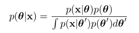
Different choices of prior can make the integral more or less difficult to calculate. If the likelihood p(x|teta) has the same algebraic form as the prior, we can obtain a closed-form expression for the posterior. This blog provides a good overview of the relationships between the choice of the prior distribution (beta/gamma) and the sampling posterior distribution.

 

Resources

 

https://onlinelibrary.wiley.com/doi/pdf/10.1002/9781119197096.app03

https://probabilityandstats.wordpress.com/tag/poisson-gamma-mixture/

https://www.johndcook.com/blog/conjugate_prior_diagram/

Original. Reposted with permission.

 

Bio: Madalina Ciortan is an academic researcher and data scientists who studies high dimensional data clustering methods with a main focus on error tolerant subspace clustering models. Madalina's work is applied on topics such as rare genetic disease analysis, cellular sub-types identification or techniques to approach biological sequencing data generation problems like dropout.

Related:

• Probability Distributions in Data Science
• What is Poisson Distribution?
• 5 Probability Distributions Every Data Scientist Should Know