Your Guide to Linear Regression Models
This article explains linear regression and how to program linear regression models in Python.
By Diego Lopez Yse, Data Scientist

Interpretability is one of the biggest challenges in machine learning. A model has more interpretability than another one if its decisions are easier for a human to comprehend. Some models are so complex and are internally structured in such a way that it’s almost impossible to understand how they reached their final results. These black boxes seem to break the association between raw data and final output, since several processes happen in between.
But in the universe of machine learning algorithms, some models are more transparent than others. Decision Trees are definitely one of them, and Linear Regression models are another one. Their simplicity and straightforward approach turns them into an ideal tool to approach different problems. Let’s see how.
You can use Linear Regression models to analyze how salaries in a given place depend on features like experience, level of education, role, city they work in, and so on. Similarly, you can analyze if real estate prices depend on factors such as their areas, numbers of bedrooms, or distances to the city center.
In this post, I’ll focus on Linear Regression models that examine the linear relationship between a dependent variable and one (Simple Linear Regression) or more (Multiple Linear Regression) independent variables.
Simple Linear Regression (SLR)
Is the simplest form of Linear Regression used when there is a single input variable (predictor) for the output variable (target):
- The input or predictor variable is the variable that helps predict the value of the output variable. It is commonly referred to as X.
- The output or target variable is the variable that we want to predict. It is commonly referred to as y.
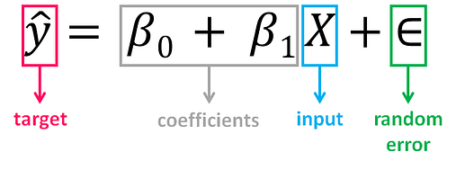
The value of β0, also called the intercept, shows the point where the estimated regression line crosses the y axis, while the value of β1 determines the slope of the estimated regression line. The random error describes the random component of the linear relationship between the dependent and independent variable (the disturbance of the model, the part of y that X is unable to explain). The true regression model is usually never known (since we are not able to capture all the effects that impact the dependent variable), and therefore the value of the random error term corresponding to observed data points remains unknown. However, the regression model can be estimated by calculating the parameters of the model for an observed data set.
The idea behind regression is to estimate the parameters β0 and β1 from a sample. If we are able to determine the optimum values of these two parameters, then we will have the line of best fit that we can use to predict the values of y, given the value of X. In other words, we try to fit a line to observe a relationship between the input and output variables and then further use it to predict the output of unseen inputs.
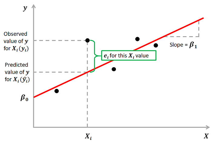
How do we estimate β0 and β1? We can use a method called Ordinary Least Squares (OLS). The goal behind this is to minimize the distance from the black dots to the red line as close to zero as possible, which is done by minimizing the squared differences between actual and predicted outcomes.
The difference between actual and predicted values is called residual (e) and can be negative or positive depending on whether the model overpredicted or underpredicted the outcome. Hence, to calculate the net error, adding all the residuals directly can lead to the cancellations of terms and reduction of the net effect. To avoid this, we take the sum of squares of these error terms, which is called the Residual Sum of Squares (RSS).
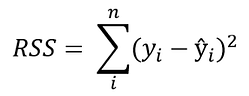
The Ordinary Least Squares (OLS) method minimizes the residual sum of squares, and its objective is to fit a regression line that would minimize the distance (measured in quadratic values) from the observed values to the predicted ones (the regression line).
Multiple Linear Regression (MLR)
Is the form of Linear Regression used when there are two or more predictors or input variables. Similar to the SLR model described before, it includes additional predictors:
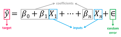
Notice that the equation is just an extension of the Simple Linear Regression one, in which each input/ predictor has its corresponding slope coefficient (β). The first β term (β0) is the intercept constant and is the value of y in absence of all predictors (i.e when all X terms are 0).
As the number of features grows, the complexity of our model increases and it becomes more difficult to visualize, or even comprehend, our data. Because there are more parameters in these models compared to SLR ones, more care is needed. when working with them. Adding more terms will inherently improve the fit to the data, but the new terms may not have any real significance. This is dangerous because it can lead to a model that fits that data but doesn’t actually mean anything useful.
An example
The advertising dataset consists of the sales of a product in 200 different markets, along with advertising budgets for three different media: TV, radio, and newspaper. We’ll use the dataset to predict the amount of sales (dependent variable), based on the TV, radio and newspaper advertising budgets (independent variables).
Mathematically, the formula we’ll try solve is:

Finding the values of these constants (β) is what regression model does by minimizing the error function and fitting the best line or hyperplane (depending on the number of input variables). Let’s code.
Load data and describe dataset
You can download the dataset under this link. Before loading the data, we’ll import the necessary libraries:
import pandas as pd
import numpy as np
import seaborn as sns
import matplotlib.pyplot as plt
from sklearn.model_selection import train_test_split
from sklearn.linear_model import LinearRegression
from sklearn import metrics
from sklearn.metrics import r2_score
import statsmodels.api as sm
Now we load the dataset:
df = pd.read_csv(“Advertising.csv”)Let’s understand the dataset and describe it:
df.head()
We’ll drop the first column (“Unnamed”) since we don’t need it:
df = df.drop([‘Unnamed: 0’], axis=1)
df.info()
Our dataset now contains 4 columns (including the target variable “sales”), 200 registers and no missing values. Let’s visualize the relationship between the independent and target variables.
sns.pairplot(df)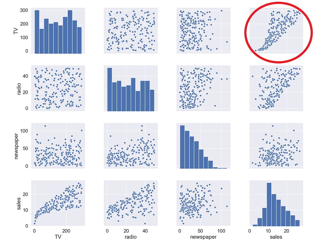
The relationship between TV and sales seems to be pretty strong, and while there seems to be some trend between radio and sales, the relationship between newspaper and sales seems to be nonexistent. We can verify that also numerically through a correlation map:
mask = np.tril(df.corr())
sns.heatmap(df.corr(), fmt=’.1g’, annot=True, cmap= ‘cool’, mask=mask)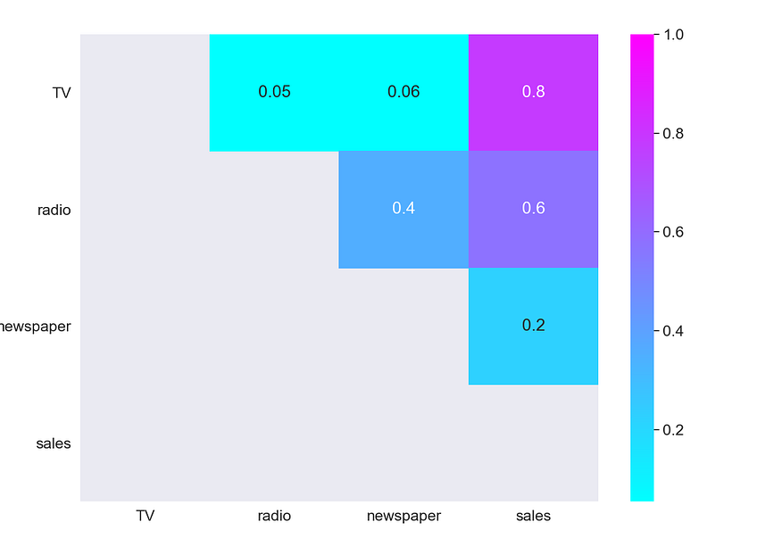
As we expected, the strongest positive correlation happens between sales and TV, while the relationship between sales and newspaper is close to 0.
Select features and target variable
Next, we divide the variables into two sets: dependent (or target variable “y”) and independents (or feature variables “X”)
X = df.drop([‘sales’], axis=1)
y = df[‘sales’]
Split the dataset
To understand model performance, dividing the dataset into a training set and a test set is a good strategy. By splitting the dataset into two separate sets, we can train using one set and test the model performance using unseen data on the other one.
X_train, X_test, y_train, y_test = train_test_split(X, y, test_size=0.3, random_state=0)We split our dataset into 70% train and 30% test. The random_state parameter is used for initializing the internal random number generator, which will decide the splitting of data into train and test indices in your case. I set random state = 0 so that you can compare your output over multiple runs of the code using the same parameter.
print(X_train.shape,y_train.shape,X_test.shape,y_test.shape)
By printing the shape of the splitted sets, we see that we created:
- 2 datasets of 140 registers each (70% of total registers), one with 3 independent variables and one with just the target variable, that will be used for training and producing the linear regression model.
- 2 datasets of 60 registers each (30% of total registers), one with 3 independent variables and one with just the target variable, that will be used for testing the performance of the linear regression model.
Build model
Building the model is as simple as:
mlr = LinearRegression()
Train model
Fitting your model to the training data represents the training part of the modelling process. After it is trained, the model can be used to make predictions, with a predict method call:
mlr.fit(X_train, y_train)Let’s see the output of the model after being trained, and take a look at the value of β0 (the intercept):
mlr.intercept_
We can also print the values of the coefficients (β):
coeff_df = pd.DataFrame(mlr.coef_, X.columns, columns =[‘Coefficient’])
coeff_df
This way we can now estimate the value of “sales” based on different budget values for TV, radio and newspaper:

For example, if we determine a budget value of 50 for TV, 30 for radio and 10 for newspaper, the estimated value of “sales” will be:
example = [50, 30, 10]
output = mlr.intercept_ + sum(example*mlr.coef_)
output
Test model
A test dataset is a dataset that is independent of the training dataset. This test dataset is the unseen data set for your model which will help you have a better view of its ability to generalize:
y_pred = mlr.predict(X_test)
Evaluate Performance
The quality of a model is related to how well its predictions match up against the actual values of the testing dataset:
print(‘Mean Absolute Error:’, metrics.mean_absolute_error(y_test, y_pred))
print(‘Mean Squared Error:’, metrics.mean_squared_error(y_test, y_pred))
print(‘Root Mean Squared Error:’, np.sqrt(metrics.mean_squared_error(y_test, y_pred)))
print(‘R Squared Score is:’, r2_score(y_test, y_pred))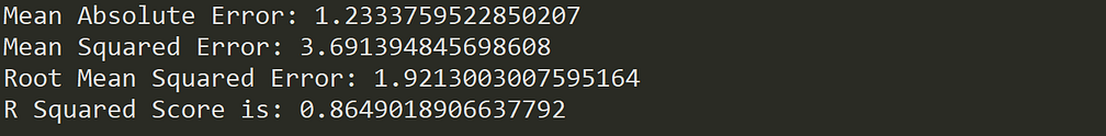
After validating our model against the testing set, we get an R² of 0.86 which seems like a pretty decent performance score. But although a higher R² indicates a better fit for the model, it’s not always the case that a high measure is a positive thing. We’ll see below some ways to interpret and improve our regression models.
How to interpret and improve your model?
OK, we created our model, and now what? Let’s take a look at the model statistics over the training data to get some answers:
X2 = sm.add_constant(X_train)
model_stats = sm.OLS(y_train.values.reshape(-1,1), X2).fit()
model_stats.summary()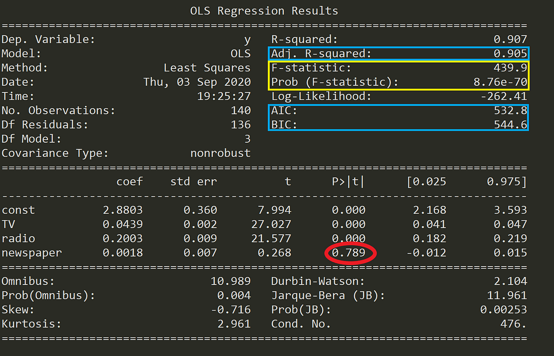
Let’s see below what these numbers mean.
Hypothesis Test
One of the fundamental questions you should answer while running a MLR model is, whether or not, at least one of the predictors is useful in predicting the output. What if the relationship between the independent variables and target is just by chance and there is no actual impact on sales due to any of the predictors?
We need to perform a Hypothesis Test to answer this question and check our assumptions. It all starts by forming a Null Hypothesis (H0), which states that all the coefficients are equal to zero, and there’s no relationship between predictors and target (meaning that a model with no independent variables fits the data as well as your model):
On the other hand, we need to define an Alternative Hypothesis (Ha), which states that at least one of the coefficients is not zero, and there is a relationship between predictors and target (meaning that your model fits the data better than the intercept-only model):

If we want to reject the Null Hypothesis and have confidence in our regression model, we need to find strong statistical evidence. To do this we perform a hypothesis test, for which we use the F-Statistic.
If the value of F-statistic is equal to or very close to 1, then the results are in favor of the Null Hypothesis and we fail to reject it.
As we can see in the table above (marked in yellow), the F-statistic is 439.9, thus providing strong evidence against the Null Hypothesis (that all coefficients are zero). Next, we also need to check the probability of occurrence of the F-statistic (also marked in yellow) under the assumption that the null hypothesis is true, which is 8.76e-70, an exceedingly small number lower than 1%. This means that there is much less than 1% probability that the F-statistic of 439.9 could have occurred by chance under the assumption of a valid Null hypothesis.
Having said this, we can reject the Null Hypothesis and be confident that at least one predictor is useful in predicting the output.
Generate models
Running a Linear Regression model with many variables including irrelevant ones will lead to a needlessly complex model. Which of the predictors are important? Are all of them significant to our model? To find that out, we need to perform a process called feature selection. The 2 main methods for feature selection are:
- Forward Selection: where predictors are added one at a time beginning with the predictor with the highest correlation with the dependent variable. Then, variables of greater theoretical importance are incorporated to the model sequentially, until a stopping rule is reached.
- Backward Elimination: where you start with all variables in the model, and remove the variables that have the least statistically significant (greater p-value), until a stopping rule is reached.
Although both methods can be used, unless the number of predictors is larger than the sample size (or number of events), it’s usually preferred to use a backward elimination approach.
You can find a full example and implementation of these methods in this link.
Compare models
Every time you add an independent variable to a model, the R² increases, even if the independent variable is insignificant. In our model, are all predictors contributing to an increase in sales? And if so, are they all doing it in the same extent?
As opposed to R², Adjusted R² is a measure that increases only when the independent variable is significant and affects the dependent variable. So,if your R² score increases but the Adjusted R² score decreases as you add variables to the model, then you know that some features are not useful and you should remove them.
An interesting finding in the table above is that the p-value for newspaper is super high (0.789, marked in red). Finding the p-value for each coefficient will tell if the variable is statistically significant to predict the target or not.
As a general rule of thumb, if the p-value for a given variable is less than 0.05 then there is a strong relationship between that variable and the target.
This way, including the variable newspaper doesn’t seem to be appropriate to reach a robust model, and removing it may improve the performance and generalization of the model.
Besides Adjusted R² score you can use other criteria to compare different regression models:
- Akaike Information Criterion (AIC): is a technique used to estimate the likelihood of a model to predict/estimate the future values. It rewards models that achieve a high goodness-of-fit score and penalizes them if they become overly complex. A good model is the one that has minimum AIC among all the other models.
- Bayesian Information Criterion (BIC): is another criteria for model selection that measures the trade-off between model fit and complexity, penalizing overly complex models even more than AIC.
Assumptions
Because Linear Regression models are an approximation of the long-term sequence of any event, they require some assumptions to be made about the data they represent in order to remain appropriate. Most statistical tests rely upon certain assumptions about the variables used in the analysis, and when these assumptions are not met, the results may not be trustworthy (e.g. resulting in Type I or Type II errors).
Linear Regression models are linear in the sense that the output is a linear combination of the input variables, and only suited for modeling linearly separable data. Linear Regression models work under various assumptions that must be present in order to produce a proper estimation and not to depend solely on accuracy scores:
- Linearity: the relationship between the features and target must be linear. One way to check the linear relationships is to visually inspect scatter plots for linearity. If the relationship displayed in the scatter plot is not linear, then we’d need to run a non-linear regression or transform the data.
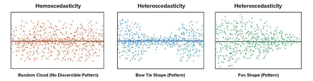
- Homoscedasticity: the variance of the residual must be the same for any value of x. Multiple linear regression assumes that the amount of error in the residuals is similar at each point of the linear model. This scenario is known as homoscedasticity. Scatter plots are a good way to check whether the data are homoscedastic, and also several tests exist to validate the assumption numerically (e.g. Goldfeld-Quandt, Breusch-Pagan, White)
- No multicollinearity: data should not show multicollinearity, which occurs when the independent variables (explanatory variables) are highly correlated to one another. If this happens, there will be problems in figuring out the specific variable that contributes to the variance in the dependent/target variable. This assumption can be tested with the Variance Inflation Factor (VIF) method, or through a correlation matrix. Alternatives to solve this issue may be centering the data (deducting the mean score), or conducting a factor analysis and rotating the factors to insure independence of the factors in the linear regression analysis.
- No autocorrelation: the value of the residuals should be independent of one another. The presence of correlation in residuals drastically reduces model’s accuracy. If the error terms are correlated, the estimated standard errors tend to underestimate the true standard error. To test for this assumption, you can use the Durbin-Watson statistic.
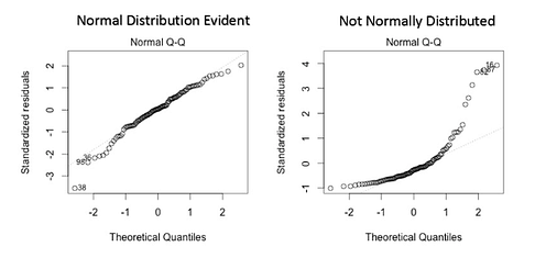
- Normality of residuals: residuals must be normally distributed. Normality can be checked with a goodness of fit test (e.g. Kolmogorov-Smirnov or Shapiro-Wilk tests), and if data is not normally distributed, a non-linear transformation (e.g. log transformation) might fix the issue.
Assumptions are critical because if they are not valid, then the analytical process can be considered unreliable, unpredictable, and out of control. Failing to meet the assumptions can lead to draw conclusions that are not valid or scientifically unsupported by the data.
You can find a full testing of the assumptions in this link.
Final thoughts
Although MLR models extend the scope of SLR models, they are still linear models, meaning that the terms included in the model are incapable of showing any non-linear relationships between each other or representing any sort of non-linear trend. You should also be careful when predicting a point outside the observed range of features since the relationship among variables may change as you move outside the observed range (a fact that you can’t know because you don’t have the data).
The observed relationship may be locally linear, but there may be unobserved non-linear relationships on the outside range of your data.
Linear models can also model curvatures by including non-linear variables such as polynomials and transforming exponential functions. The linear regression equation is linear in the parameters, meaning you can raise an independent variable by an exponent to fit a curve, and still remain in the “linear world”. Linear Regression models can contain log terms and inverse terms to follow different kinds of curves and yet continue to be linear in the parameters.

Regressions like Polynomial Regression can model non-linear relationships, and while a linear equation has one basic form, non-linear equations can take many different forms. The reason you might consider using Non-linear Regression Models is that, while linear regression can model curves, it might not be able to model the specific curve that exists in your data.
You should also know that OLS is not the only method to fit your Linear Regression model, and other optimization methods like Gradient Descent are more adequate to fit large datasets. Applying OLS to complex and non-linear algorithms might not be scalable, and Gradient Descent can be computationally cheaper (faster) for finding the solution. Gradient Descent is an algorithm that minimizes functions, and given a function defined by a set of parameters, the algorithm starts with an initial set of parameter values and iteratively moves toward a set of parameter values that minimize the function. This iterative minimization is achieved using derivatives, taking steps in the negative direction of the function gradient.
Another key thing to take into account is that outliers can have a dramatic effect on regression lines and the correlation coefficient. In order to identify them it’s essential to perform Exploratory Data Analysis (EDA), examining the data to detect unusual observations, since they can impact the results of our analysis and statistical modeling in a drastic way. In case you recognize any, outliers can be imputed (e.g. with mean / median / mode), capped (replacing those outside certain limits), or replaced by missing values and predicted.
Finally, some limitations of Linear Regression models are:
- Omitted variables. It is necessary to have a good theoretical model to suggest variables that explain the dependent variable. In the case of a simple two-variable regression, one has to think of other factors that might explain the dependent variable, since there may be other “unobserved” variables that explain the output.
- Reverse causality. Many theoretical models predict bidirectional causality — that is, a dependent variable can cause changes in one or more explanatory variables. For instance, higher earnings may enable people to invest more in their own education, which, in turn, raises their earnings. This complicates the way regressions should be estimated, calling for special techniques.
- Mismeasurement. Factors might be measured incorrectly. For example, aptitude is difficult to measure, and there are well-known problems with IQ tests. As a result, the regression using IQ might not properly control for aptitude, leading to inaccurate or biased correlations between variables like education and earnings.
- Too limited a focus. A regression coefficient provides information only about how small changes — not large changes — in one variable relate to changes in another. It will show how a small change in education is likely to affect earnings but it will not allow the researcher to generalize about the effect of large changes. If everyone became college educated at the same time, a newly minted college graduate would be unlikely to earn a great deal more because the total supply of college graduates would have increased dramatically.
Interested in these topics? Follow me on Linkedin or Twitter
Bio: Diego Lopez Yse is an experienced professional with a solid international background acquired in different industries (capital markets, biotechnology, software, consultancy, government, agriculture). Always a team member. Skilled in Business Management, Analytics, Finance, Risk, Project Management and Commercial Operations. MS in Data Science and Corporate Finance.
Original. Reposted with permission.
Related:
- Which methods should be used for solving linear regression?
- Before Probability Distributions
- Time Complexity: How to measure the efficiency of algorithms