Which methods should be used for solving linear regression?

By Ahmad Bin Shafiq, Machine Learning Student.

Linear Regression is a supervised machine learning algorithm. It predicts a linear relationship between an independent variable (y), based on the given dependant variables (x), such that the independent variable (y) has the lowest cost.

Different approaches to solve linear regression models

There are many different methods that we can apply to our linear regression model in order to make it more efficient. But we will discuss the most common of them here.

1. Gradient Descent
2. Least Square Method / Normal Equation Method
3. Adams Method
4. Singular Value Decomposition (SVD)

Okay, so let’s begin…

Gradient Descent

One of the most common and easiest methods for beginners to solve linear regression problems is gradient descent.

How Gradient Descent works

Now, let's suppose we have our data plotted out in the form of a scatter graph, and when we apply a cost function to it, our model will make a prediction. Now this prediction can be very good, or it can be far away from our ideal prediction (meaning its cost will be high). So, in order to minimize that cost (error), we apply gradient descent to it.

Now, gradient descent will slowly converge our hypothesis towards a global minimum, where the cost would be lowest. In doing so, we have to manually set the value of alpha, and the slope of the hypothesis changes with respect to our alpha’s value. If the value of alpha is large, then it will take big steps. Otherwise, in the case of small alpha, our hypothesis would converge slowly and through small baby steps.

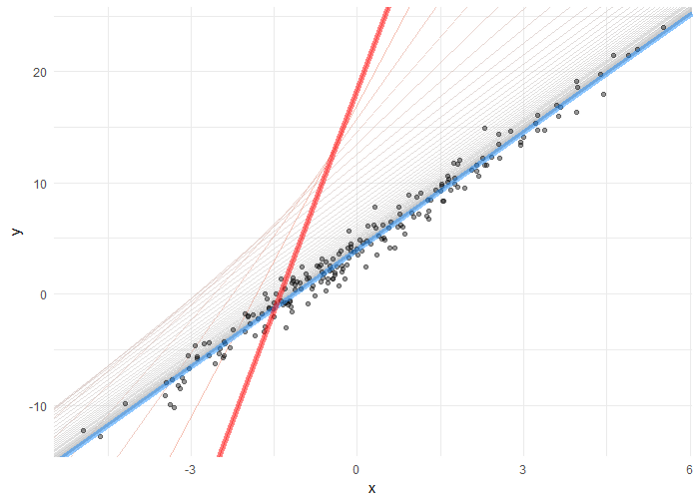
Hypothesis converging towards a global minimum. Image from Medium.

The Equation for Gradient Descent is

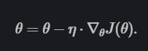
Source: Ruder.io.

Implementing Gradient Descent in Python

import numpy as np
from matplotlib import pyplot

#creating our data
X = np.random.rand(10,1)
y = np.random.rand(10,1)
m = len(y)
theta = np.ones(1)

#applying gradient descent
a = 0.0005
cost_list = []
for i in range(len(y)):
    
    theta = theta - a*(1/m)*np.transpose(X)@(X@theta - y)
           
    cost_val = (1/m)*np.transpose(X)@(X@theta - y)
    cost_list.append(cost_val)

#Predicting our Hypothesis
b = theta
yhat = X.dot(b)

#Plotting our results
pyplot.scatter(X, y, color='red')
pyplot.plot(X, yhat, color='blue')
pyplot.show()

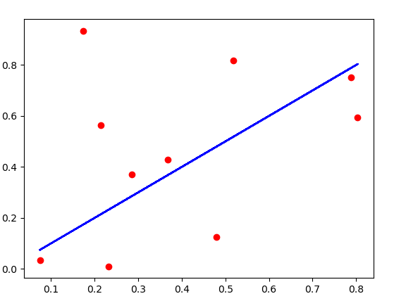
Model after Gradient Descent.

Here first, we have created our dataset, and then we looped over all our training examples in order to minimize our cost of hypothesis.

Pros:

Important advantages of Gradient Descent are

• Less Computational Cost as compared to SVD or ADAM
• Running time is O(kn²)
• Works well with more number of features

Cons:

Important cons of Gradient Descent are

• Need to choose some learning rate α
• Needs many iterations to converge
• Can be stuck in Local Minima
• If not proper Learning Rate α, then it might not converge.

Least Square Method

The least-square method, also known as the normal equation, is also one of the most common approaches to solving linear regression models easily. But, this one needs to have some basic knowledge of linear algebra.

How the least square method works

In normal LSM, we solve directly for the value of our coefficient. In short, in one step, we reach our optical minimum point, or we can say only in one step we fit our hypothesis to our data with the lowest cost possible.

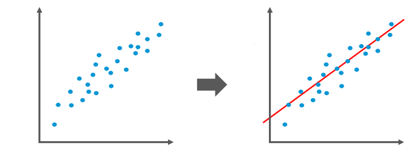
Before and after applying LSM to our dataset. Image from Medium.

The equation for LSM is

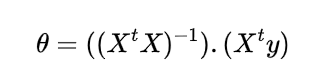
Implementing LSM in Python

import numpy as np
from matplotlib import pyplot

#creating our data
X = np.random.rand(10,1)
y = np.random.rand(10,1)

#Computing coefficient
b = np.linalg.inv(X.T.dot(X)).dot(X.T).dot(y)

#Predicting our Hypothesis
yhat = X.dot(b)
#Plotting our results
pyplot.scatter(X, y, color='red')
pyplot.plot(X, yhat, color='blue')
pyplot.show()

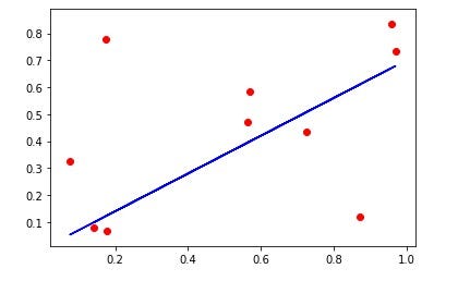
Here first we have created our dataset and then minimized the cost of our hypothesis using the

b = np.linalg.inv(X.T.dot(X)).dot(X.T).dot(y)

code, which is equivalent to our equation.

Pros:

Important advantages of LSM are:

• No Learning Rate
• No Iterations
• Feature Scaling Not Necessary
• Works really well when the Number of Features is less.

Cons:

Important cons are:

• Is computationally expensive when the dataset is big.
• Slow when Number of Features is more
• Running Time is O(n³)
• Sometimes, your X transpose X is non-invertible, i.e., a singular matrix with no inverse. You can use np.linalg.pinv instead of np.linalg.inv to overcome this problem.

Adam’s Method

ADAM, which stands for Adaptive Moment Estimation, is an optimization algorithm that is widely used in Deep Learning.

It is an iterative algorithm that works well on noisy data.

It is the combination of RMSProp and Mini-batch Gradient Descent algorithms.

In addition to storing an exponentially decaying average of past squared gradients like Adadelta and RMSprop, Adam also keeps an exponentially decaying average of past gradients, similar to momentum.

We compute the decaying averages of past and past squared gradients respectively as follows:

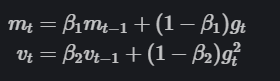
Credit: Ruder.io.

As mt and vt are initialized as vectors of 0’s, the authors of Adam observe that they are biased towards zero, especially during the initial time steps, and especially when the decay rates are small (i.e., β1β1 and β2β2 are close to 1).

They counteract these biases by computing bias-corrected first and second-moment estimates:

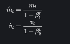
Credit: Ruder.io.

They then update the parameters with:

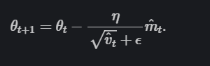
Credit: Ruder.io.

You can learn the theory behind Adam here or here.

Pseudocode for Adam is

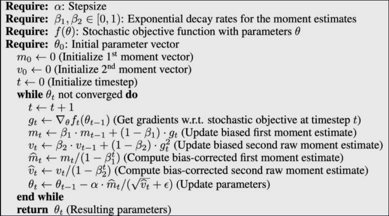
Source: Arxiv Adam.

Let’s see it’s code in Pure Python.

#Creating the Dummy Data set and importing libraries
import math
import seaborn as sns
import numpy as np 
from scipy import stats
from matplotlib import pyplot
x = np.random.normal(0,1,size=(100,1))
y = np.random.random(size=(100,1))

Now Let’s find the actual graph of Linear Regression and values for slope and intercept for our dataset.

print("Intercept is " ,stats.mstats.linregress(x,y).intercept)
print("Slope is ", stats.mstats.linregress(x,y).slope)

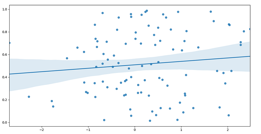
Now let us see the Linear Regression line using the Seaborn regplot function.

pyplot.figure(figsize=(15,8))
sns.regplot(x,y)
pyplot.show()

Let us code Adam Optimizer now in pure Python.

h = lambda theta_0, theta_1, x: theta_0 + np.dot(x,theta_1) #equation of straight lines

# the cost function (for the whole batch. for comparison later)
def J(x, y, theta_0, theta_1):
    m = len(x)
    returnValue = 0
    for i in range(m):
        returnValue += (h(theta_0, theta_1, x[i]) - y[i])**2
    returnValue = returnValue/(2*m)
    return returnValue

# finding the gradient per each training example
def grad_J(x, y, theta_0, theta_1):
    returnValue = np.array([0., 0.])
    returnValue[0] += (h(theta_0, theta_1, x) - y)
    returnValue[1] += (h(theta_0, theta_1, x) - y)*x
    return returnValue

class AdamOptimizer:
    def __init__(self, weights, alpha=0.001, beta1=0.9, beta2=0.999, epsilon=1e-8):
        self.alpha = alpha
        self.beta1 = beta1
        self.beta2 = beta2
        self.epsilon = epsilon
        self.m = 0
        self.v = 0
        self.t = 0
        self.theta = weights
        
    def backward_pass(self, gradient):
        self.t = self.t + 1
        self.m = self.beta1*self.m + (1 - self.beta1)*gradient
        self.v = self.beta2*self.v + (1 - self.beta2)*(gradient**2)
        m_hat = self.m/(1 - self.beta1**self.t)
        v_hat = self.v/(1 - self.beta2**self.t)
        self.theta = self.theta - self.alpha*(m_hat/(np.sqrt(v_hat) - self.epsilon))
        return self.theta

Here, we have implemented all the equations mentioned in the pseudocode above using an object-oriented approach and some helper functions.

Let us now set the hyperparameters for our model.

epochs = 1500
print_interval = 100
m = len(x)
initial_theta = np.array([0., 0.]) # initial value of theta, before gradient descent
initial_cost = J(x, y, initial_theta[0], initial_theta[1])

theta = initial_theta
adam_optimizer = AdamOptimizer(theta, alpha=0.001)
adam_history = [] # to plot out path of descent
adam_history.append(dict({'theta': theta, 'cost': initial_cost})#to check theta and cost function

And finally, the training process.

for j in range(epochs):
    for i in range(m):
        gradients = grad_J(x[i], y[i], theta[0], theta[1])
        theta = adam_optimizer.backward_pass(gradients)
    
    if ((j+1)%print_interval == 0 or j==0):
        cost = J(x, y, theta[0], theta[1])
        print ('After {} epochs, Cost = {}, theta = {}'.format(j+1, cost, theta))
        adam_history.append(dict({'theta': theta, 'cost': cost}))
        
print ('\nFinal theta = {}'.format(theta))

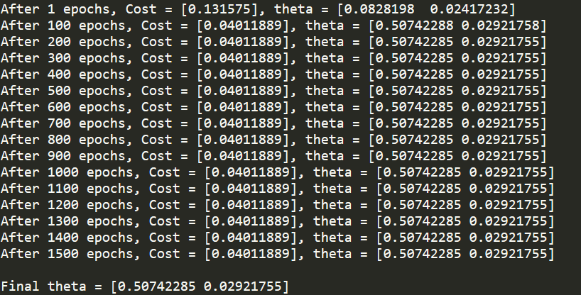
Now, if we compare the Final theta values to the slope and intercept values, calculated earlier using scipy.stats.mstat.linregress, they are almost 99% equal and can be 100% equal by adjusting the hyperparameters.

Finally, let us plot it.

b = theta
yhat = b[0] + x.dot(b[1])
pyplot.figure(figsize=(15,8))
pyplot.scatter(x, y, color='red')
pyplot.plot(x, yhat, color='blue')
pyplot.show()

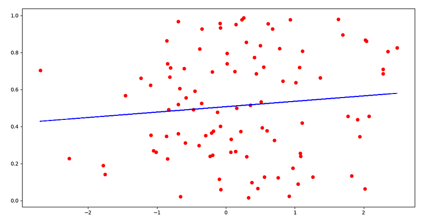
And we can see that our plot is similar to plot obtained using sns.regplot.

Pros:

• Straightforward to implement.
• Computationally efficient.
• Little memory requirements.
• Invariant to diagonal rescale of the gradients.
• Well suited for problems that are large in terms of data and/or parameters.
• Appropriate for non-stationary objectives.
• Appropriate for problems with very noisy/or sparse gradients.
• Hyper-parameters have intuitive interpretation and typically require little tuning.

Cons:

• Adam and RMSProp are highly sensitive to certain values of the learning rate (and, sometimes, other hyper-parameters like the batch size), and they can catastrophically fail to converge if e.g., the learning rate is too high. (Source: stackexchange)

Singular Value Decomposition

Singular value decomposition shortened as SVD is one of the famous and most widely used dimensionality reduction methods in linear regression.

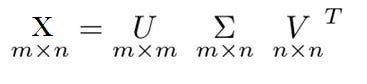
SVD is used (amongst other uses) as a preprocessing step to reduce the number of dimensions for our learning algorithm. SVD decomposes a matrix into a product of three other matrices (U, S, V).

Once our matrix has been decomposed, the coefficients for our hypothesis can be found by calculating the pseudoinverse of the input matrix X and multiplying that by the output vector y. After that, we fit our hypothesis to our data, and that gives us the lowest cost.

Implementing SVD in Python

import numpy as np
from matplotlib import pyplot

#Creating our data
X = np.random.rand(10,1)
y = np.random.rand(10,1)

#Computing coefficient
b = np.linalg.pinv(X).dot(y)

#Predicting our Hypothesis
yhat = X.dot(b)

#Plotting our results
pyplot.scatter(X, y, color='red')
pyplot.plot(X, yhat, color='blue')
pyplot.show()

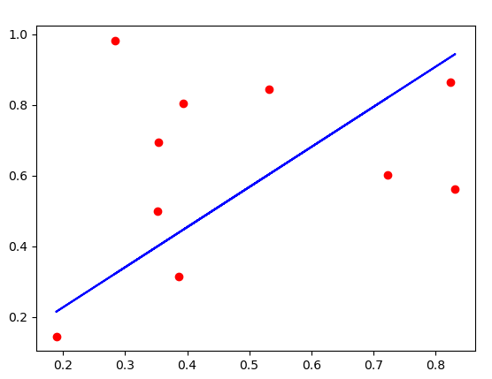
Though it is not converged very well, it is still pretty good.

Here first, we have created our dataset and then minimized the cost of our hypothesis using b = np.linalg.pinv(X).dot(y), which is the equation for SVD.

Pros:

• Works better with higher dimensional data
• Good for gaussian type distributed data
• Really stable and efficient for a small dataset
• While solving linear equations for linear regression, it is more stable and the preferred approach.

Cons:

• Running time is O(n³)
• Multiple risk factors
• Really sensitive to outliers
• May get unstable with a very large dataset

Learning Outcome

As of now, we have learned and implemented gradient descent, LSM, ADAM, and SVD. And now, we have a very good understanding of all of these algorithms, and we also know what are the pros and cons.

One thing we noticed was that the ADAM optimization algorithm was the most accurate, and according to the actual ADAM research paper, ADAM outperforms almost all other optimization algorithms.

Related:

• Linear to Logistic Regression, Explained Step by Step
• A Beginner’s Guide to Linear Regression in Python with Scikit-Learn
• Linear Regression In Real Life