
 Essential Linear Algebra for Data Science and Machine Learning

 Essential Linear Algebra for Data Science and Machine Learning
Linear algebra is foundational in data science and machine learning. Beginners starting out along their learning journey in data science--as well as established practitioners--must develop a strong familiarity with the essential concepts in linear algebra.
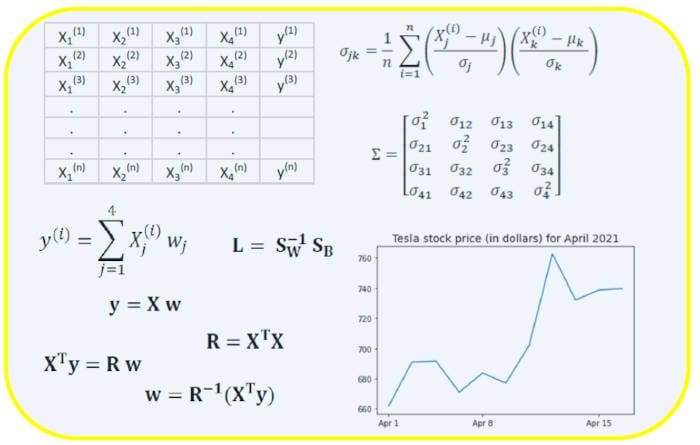
Image by Benjamin O. Tayo.
Linear Algebra is a branch of mathematics that is extremely useful in data science and machine learning. Linear algebra is the most important math skill in machine learning. Most machine learning models can be expressed in matrix form. A dataset itself is often represented as a matrix. Linear algebra is used in data preprocessing, data transformation, and model evaluation. Here are the topics you need to be familiar with:
- Vectors
- Matrices
- Transpose of a matrix
- Inverse of a matrix
- Determinant of a matrix
- Trace of a matrix
- Dot product
- Eigenvalues
- Eigenvectors
In this article, we illustrate the application of linear algebra in data science and machine learning using the tech stocks dataset, which can be found here.
1. Linear Algebra for Data Preprocessing
We begin by illustrating how linear algebra is used in data preprocessing.
1.1 Import necessary libraries for linear algebra
import numpy as np
import pandas as pd
import pylab
import matplotlib.pyplot as plt
import seaborn as sns
1.2 Read dataset and display features
data = pd.read_csv("tech-stocks-04-2021.csv")
data.head()
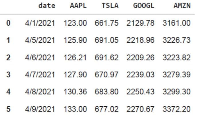
Table 1. Stock prices for selected stock prices for the first 16 days in April 2021.
print(data.shape)
output = (11,5)
The data.shape function enables us to know the size of our dataset. In this case, the dataset has 5 features (date, AAPL, TSLA, GOOGL, and AMZN), and each feature has 11 observations. Date refers to the trading days in April 2021 (up to April 16). AAPL, TSLA, GOOGL, and AMZN are the closing stock prices for Apple, Tesla, Google, and Amazon, respectively.
1.3 Data visualization
To perform data visualization, we would need to define column matrices for the features to be visualized:
x = data['date']
y = data['TSLA']
plt.plot(x,y)
plt.xticks(np.array([0,4,9]), ['Apr 1','Apr 8','Apr 15'])
plt.title('Tesla stock price (in dollars) for April 2021',size=14)
plt.show()
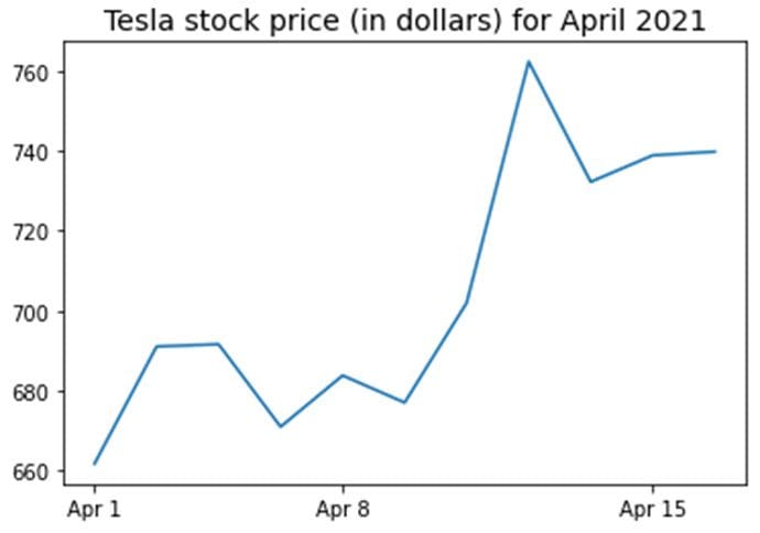
Figure 1. Tesla stock price for first 16 days in April 2021.
2. Covariance Matrix
The covariance matrix is one of the most important matrices in data science and machine learning. It provides information about co-movement (correlation) between features. Suppose we have a features matrix with 4 features and n observations as shown in Table 2:
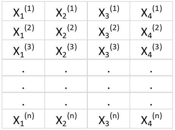
Table 2. Features matrix with 4 variables and n observations.
To visualize the correlations between the features, we can generate a scatter pairplot:
cols=data.columns[1:5]
print(cols)
output = Index(['AAPL', 'TSLA', 'GOOGL', 'AMZN'], dtype='object')
sns.pairplot(data[cols], height=3.0)
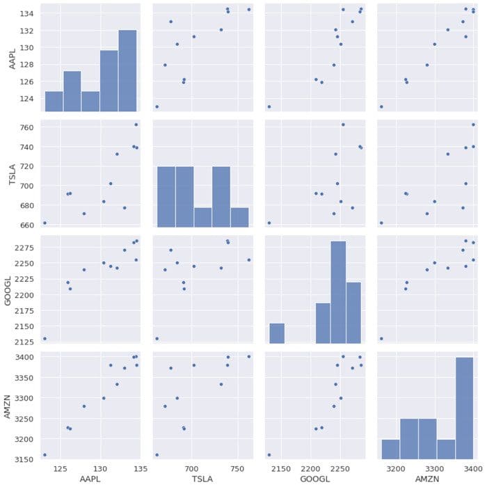
Figure 2. Scatter pairplot for selected tech stocks.
To quantify the degree of correlation between features (multicollinearity), we can compute the covariance matrix using this equation:
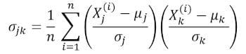
where and are the mean and standard deviation of feature , respectively. This equation indicates that when features are standardized, the covariance matrix is simply the dot product between features.
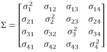
In matrix form, the covariance matrix can be expressed as a 4 x 4 real and symmetric matrix:
This matrix can be diagonalized by performing a unitary transformation, also referred to as Principal Component Analysis (PCA) transformation, to obtain the following:
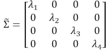
Since the trace of a matrix remains invariant under a unitary transformation, we observe that the sum of the eigenvalues of the diagonal matrix is equal to the total variance contained in features X1, X2, X3, and X4.
2.1 Computing the covariance matrix for tech stocks
from sklearn.preprocessing import StandardScaler
stdsc = StandardScaler()
X_std = stdsc.fit_transform(data[cols].iloc[:,range(0,4)].values)
cov_mat = np.cov(X_std.T, bias= True)
Note that this uses the transpose of the standardized matrix.
2.2 Visualization of covariance matrix
plt.figure(figsize=(8,8))
sns.set(font_scale=1.2)
hm = sns.heatmap(cov_mat,
                 cbar=True,
                 annot=True,
                 square=True,
                 fmt='.2f',
                 annot_kws={'size': 12},
                 yticklabels=cols,
                 xticklabels=cols)
plt.title('Covariance matrix showing correlation coefficients')
plt.tight_layout()
plt.show()
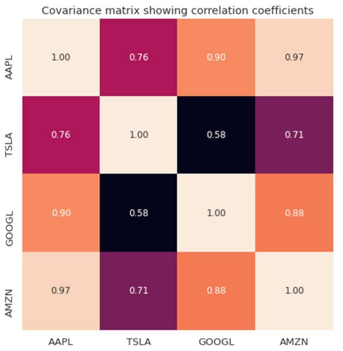
Figure 3. Covariance matrix plot for selected tech stocks.
We observe from Figure 3 that AAPL correlates strongly with GOOGL and AMZN, and weakly with TSLA. TSLA correlates generally weakly with AAPL, GOOGL and AMZN, while AAPL, GOOGL, and AMZN correlate strongly among each other.
2.3 Compute eigenvalues of the covariance matrix
np.linalg.eigvals(cov_mat)
output = array([3.41582227, 0.4527295 , 0.02045092, 0.11099732])
np.sum(np.linalg.eigvals(cov_mat))
output = 4.000000000000006
np.trace(cov_mat)
output = 4.000000000000001
We observe that the trace of the covariance matrix is equal to the sum of the eigenvalues as expected.
2.4 Compute the cumulative variance
Since the trace of a matrix remains invariant under a unitary transformation, we observe that the sum of the eigenvalues of the diagonal matrix is equal to the total variance contained in features X1, X2, X3, and X4. Hence, we can define the following quantities:
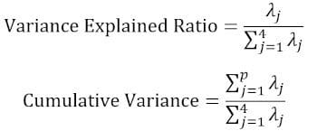
Notice that when p = 4, the cumulative variance becomes equal to 1 as expected.
eigen = np.linalg.eigvals(cov_mat)
cum_var = eigen/np.sum(eigen)
print(cum_var)
output = [0.85395557 0.11318237 0.00511273 0.02774933]

print(np.sum(cum_var))
output = 1.0
We observe from the cumulative variance (cum_var) that 85% of the variance is contained in the first eigenvalue and 11% in the second. This means when PCA is implemented, only the first two principal components could be used, as 97% of the total variance is contributed by these 2 components. This can essentially reduce the dimensionally of the feature space from 4 to 2 when PCA is implemented.
3. Linear Regression Matrix
Suppose we have a dataset that has 4 predictor features and n observations, as shown below.
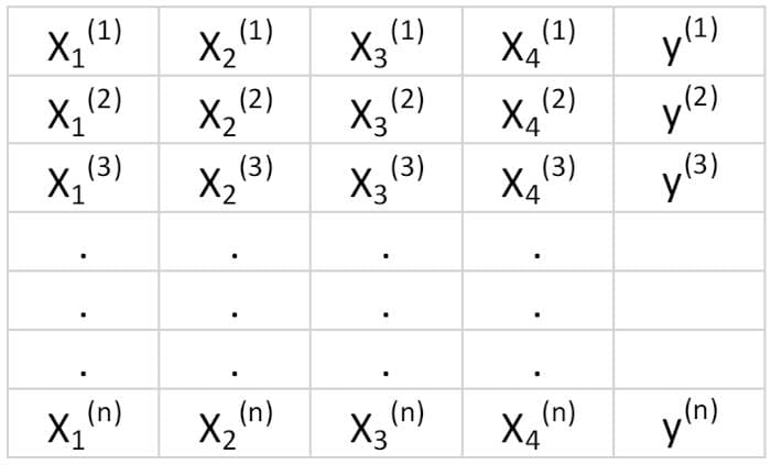
Table 3. Features matrix with 4 variables and n observations. Column 5 is the target variable (y).
We would like to build a multi-regression model for predicting the y values (column 5). Our model can thus be expressed in the form
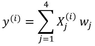
In matrix form, this equation can be written as
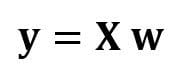
where X is the ( n x 4) features matrix, w is the (4 x 1) matrix representing the regression coefficients to be determined, and y is the (n x 1) matrix containing the n observations of the target variable y.
Note that X is a rectangular matrix, so we can’t solve the equation above by taking the inverse of X.
To convert X into a square matrix, we multiple the left-hand side and right-hand side of our equation by the transpose of X, that is
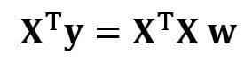
This equation can also be expressed as
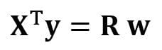
where
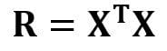
is the (4×4) regression matrix. Clearly, we observe that R is a real and symmetric matrix. Note that in linear algebra, the transpose of the product of two matrices obeys the following relationship

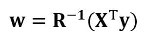
Now that we’ve reduced our regression problem and expressed it in terms of the (4×4) real, symmetric, and invertible regression matrix R, it is straightforward to show that the exact solution of the regression equation is then
Examples of regression analysis for predicting continuous and discrete variables are given in the following:
Linear Regression Basics for Absolute Beginners
Building a Perceptron Classifier Using the Least Squares Method
4. Linear Discriminant Analysis Matrix
Another example of a real and symmetric matrix in data science is the Linear Discriminant Analysis (LDA) matrix. This matrix can be expressed in the form:
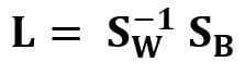
where SW is the within-feature scatter matrix, and SB is the between-feature scatter matrix. Since both matrices SW and SB are real and symmetric, it follows that L is also real and symmetric. The diagonalization of L produces a feature subspace that optimizes class separability and reduces dimensionality. Hence LDA is a supervised algorithm, while PCA is not.
For more details about the implementation of LDA, please see the following references:
Machine Learning: Dimensionality Reduction via Linear Discriminant Analysis
GitHub repository for LDA implementation using Iris dataset
Python Machine Learning by Sebastian Raschka, 3rd Edition (Chapter 5)
Summary
In summary, we’ve discussed several applications of linear algebra in data science and machine learning. Using the tech stocks dataset, we illustrated important concepts such as the size of a matrix, column matrices, square matrices, covariance matrix, transpose of a matrix, eigenvalues, dot products, etc. Linear algebra is an essential tool in data science and machine learning. Thus, beginners interested in data science must familiarize themselves with essential concepts in linear algebra.
Related: