
Image by author
What is the Pandas?
Pandas is a flexible and easy-to-use tool for performing data analysis and data manipulation. It is widely used among data scientists for preparing data, cleaning data, and running data science experiments. Pandas is an open-source library that helps you solve complex statistical problems with simple and easy-to-use syntax.
I have created a simple guide for a gentle introduction to Pandas functions. In this guide we will learn about data importing, data exporting, exploring data, data summary, selecting & filtering, sorting, renaming, dropping data, applying functions, and visualization.
Importing Data
For importing, we are going to use Kaggle’s open-source dataset Social Network Advertisements. This dataset contains three columns and 400 samples. To get started, let’s import our CSV (Comma Separated Values) file using read_csv().
import pandas as pd

data = pd.read_csv("Social_Network_Ads.csv")
type(data)

>>> pandas.core.frame.DataFrame
As we can see our CSV file has been successfully loaded and converted to Pandas Dataframes. To see the first five rows we will use head().
data.head()
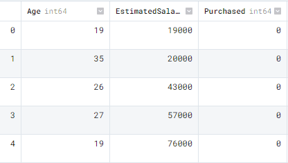
The Pandas dataframe contains Age, EstimatedSalary, and Purchased columns.
Other Formats
Apart from csv files we can import Excel files, import files from any SQL server, read and parse json files, import tables from websites using HTML parsing, and creating dataframe using dictionary. Pandas makes importing any type of data simple.
pd.read_excel('filename')
pd.read_sql(query,connection_object)
pd.read_json(json_string)
pd.read_html(url)
pd.DataFrame(dict)
Exporting Data
For exporting DataFrame into CSV we will use to_csv().
data.to_csv("new_wine_data.csv",index=False)
Similarly, we can export the dataframe into excel, send to sql, to json, and create an HTML table with one line of code.
data.to_excel(filename)
data.to_sql(table_name, connection_object)
data.to_json(filename)
data.to_html(filename)
Data Summary
To generate a simple data summary we will use the info() function. The summary includes dtypes, number of samples, and memory usage.
data.info()RangeIndex: 400 entries, 0 to 399 Data columns (total 3 columns): # Column Non-Null Count Dtype --- ------ -------------- ----- 0 Age 400 non-null int64 1 EstimatedSalary 400 non-null int64 2 Purchased 400 non-null int64 dtypes: int64(3) memory usage: 9.5 KB
Similarly, to get specific information about dataframe we can use .shape for numbers of columns and rows, .index for index range, and .columns for the names of the columns. These small utilities can come handy in solving larger data problems.
data.shape
>>> (400, 3)
data.index
>>> RangeIndex(start=0, stop=400, step=1)
data.columns
>>> Index(['Age', 'EstimatedSalary', 'Purchased'], dtype='object')
describe() will give us a summary of the distribution of numerical columns. It includes mean, standard deviation, minimum/ maximum values, and inter quartile range.
data.describe()

Age  EstimatedSalary   Purchased
count  400.000000       400.000000  400.000000
mean    37.655000     69742.500000    0.357500
std     10.482877     34096.960282    0.479864
min     18.000000     15000.000000    0.000000
25%     29.750000     43000.000000    0.000000
50%     37.000000     70000.000000    0.000000
75%     46.000000     88000.000000    1.000000
max     60.000000    150000.000000    1.000000
To check the missing values we can simile use isnull() function which will return values in boolean and we can sum them up to get exact numbers. Our dataset have zero missing values.
data.isnull().sum()
Age                0
EstimatedSalary    0
Purchased          0
dtype: int64
corr() will generate correlation matrix between numeric columns. There are no high correlation between columns.
data.corr()
                     Age  EstimatedSalary  Purchased
Age              1.000000         0.155238   0.622454
EstimatedSalary  0.155238         1.000000   0.362083
Purchased        0.622454         0.362083   1.000000
Selecting and Filtering
There are various ways to select columns. The example below is direct selection.
Use data[“<column_name>”] or data.<column_name>
data["Age"]
0      19
1      35
2      26
3      27
4      19
       ..
395    46
396    51
397    50
398    36
399    49
Name: Age, Length: 400, dtype: int64

data.Purchased.head()
0    0
1    0
2    0
3    0
4    0
Name: Purchased, dtype: int64
We can also use iloc and loc to select columns and rows as shown below.
data.iloc[0,1]
19000

data.loc[0,"Purchased"]
0
To count the number of categories in a column we will use the value_counts() function.
data.Purchased.value_counts()
0    257
1    143
Name: Purchased, dtype: int64
Filtering values is easy. We just need to give simple Python conditions. In our case, we are filtering only 1’s from the Purchased column.
print(data[data['Purchased']==1].head())
   Age  EstimatedSalary  Purchased
7    32           150000          1
16   47            25000          1
17   45            26000          1
18   46            28000          1
19   48            29000          1
For a more complex demonstration, we have added a second condition by using &.
print(data[(data['Purchased']==1) & (data['Age']>=35)])

    Age  EstimatedSalary  Purchased
16    47            25000          1
17    45            26000          1
18    46            28000          1
19    48            29000          1
20    45            22000          1
..   ...              ...        ...
393   60            42000          1
395   46            41000          1
396   51            23000          1
397   50            20000          1
399   49            36000          1

[129 rows x 3 columns]
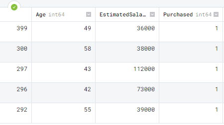
Data sorting
For sorting index we use sort_values(). It takes multiple arguments, first is the column by which we want to sort and the second is the direction of sorting. In our case, we are sorting by Purchased columns in descending order.
data.sort_values('Purchased', ascending=False).head()
sort_index() is similar to sort index but it will sort the dataframe using index numbers.
data.sort_index()
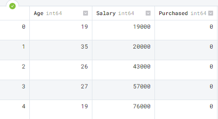
Renaming Columns
To rename a column we need a dictionary of the current and modified column name. We are changing names from ‘EstimatedSalary` to `Salary` using the rename() function.
data = data.rename(columns= {'EstimatedSalary' : 'Salary'})
data.head()
Drop Data
We can simply use the drop function to drop a column or a row. In this example, we have successfully dropped the `Salary` column.
data.drop(columns='Salary').head()

For dropping a row you can simply write a row number.
data.drop(1)
Converting Data Types
We have three columns and all of them are integers. Let’s change “Purchased” to boolean as it contains only ones and zero.
data.dtypes
Age              int64
Salary           int64
Purchased        int64
dtype: object
Use the astype() function and change the data type.
data['Purchased'] = data['Purchased'].astype('bool')
We have successfully changed the ‘Purchased’ column to boolean type.
data.dtypes
Age          int64
Salary       int64
Purchased     bool
dtype: object
Apply Functions
Applying a Python function to a column or on a whole dataset has come simpler with Pandas apply() function. In this section, we will create a simple function of doubling the values and apply it to the ‘Salary’ column.
def double(x):   #create a function
    return x*2

data['double_Salary'] = data['Salary'].apply(double)
print(data.head())
As we can observe that the newly created columns contain double the salary.
   Age  Salary  Purchased  double_Salary
0   19   19000      False          38000
1   35   20000      False          40000
2   26   43000      False          86000
3   27   57000      False         114000
4   19   76000      False         152000
We can also use the Python lambda function inside the apply function to get similar results.
data['Salary'].apply(lambda x: x*2).head()
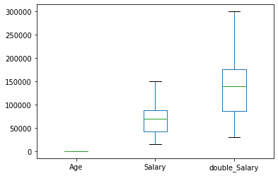
Visualization
Pandas uses matplotlib library to visualize the data. We can use this function to generate bar charts, line charts, pie charts, box plot, histogram, KDE plot and much more. We can also customize our plots similarly to the matplotlib library. By simply changing the kind of graph we can generate any type of graph using plot() function.
The box plot shows the distribution of three numerical columns.
data.plot( kind='box');
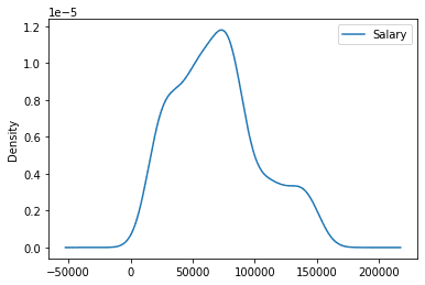
To plot density plots, we need x and y arguments and kind. In this example, we have plotted, Age versus Salary density graph.
data.plot(x="Age",y = "Salary", kind='density');
Conclusion
There is so much to Pandas that we haven't covered. It is the most used library among data scientists and data practitioners. If you are interested in learning more then check out Python Pandas Tutorial or take a proper data analytics course to learn use cases of Pandas. In this guide, we have learned about Pandas Python library and how we can use it to perform various data manipulation and analytics tasks. I hope you liked it and if you have questions related to the topics, please type them in the comment section and I will do my best to answer.
Abid Ali Awan (@1abidaliawan) is a certified data scientist professional who loves building machine learning models. Currently, he is focusing on content creation and writing technical blogs on machine learning and data science technologies. Abid holds a Master's degree in Technology Management and a bachelor's degree in Telecommunication Engineering. His vision is to build an AI product using a graph neural network for students struggling with mental illness.