An Intuitive Introduction to Gradient Descent
This post provides a good introduction to Gradient Descent, covering the intuition, variants and choosing the learning rate.
By Keshav Dhandhania and Savan Visalpara.
Gradient Descent is one of the most popular and widely used optimization algorithms. Given a machine learning model with parameters (weights and biases) and a cost function to evaluate how good a particular model is, our learning problem reduces to that of finding a good set of weights for our model which minimizes the cost function.
Gradient descent is an iterative method. We start with some set of values for our model parameters (weights and biases), and improve them slowly. To improve a given set of weights, we try to get a sense of the value of the cost function for weights similar to the current weights (by calculating the gradient) and move in the direction in which the cost function reduces. By repeating this step thousands of times we’ll continually minimize our cost function.
Pseudocode for Gradient Descent
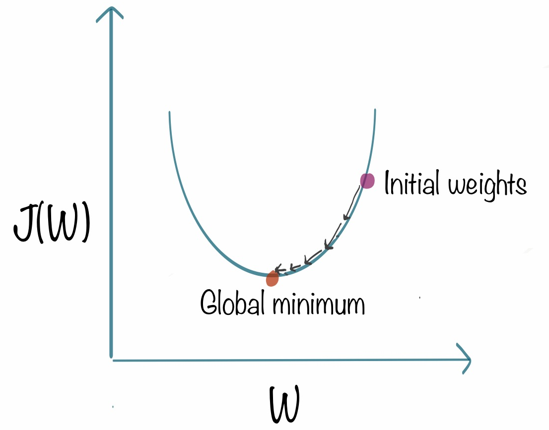
Gradient descent is used to minimize a cost function J(w) parametrized by model parameters w. The gradient (or derivative) tells us the incline or slope of the cost function. Hence, to minimize the cost function, we move in the direction opposite to the gradient.
- initializethe weights w randomly
- calculate the gradients G of cost function w.r.t parameters [1]
- update the weights by an amount proportional to G, i.e. w = w - ηG
- repeat till cost J(w) stops reducing or other pre-defined termination criteriais met
In step 3, η is the learning rate which determines the size of the steps we take to reach a minimum. We need to be very careful about this parameter since high values of η may overshoot the minimum and very low value will reach minimum very slowly.
A popular sensible choice for the termination criteria is that the cost J(w) stops reducing on the validation dataset.
Intuition for Gradient Descent
Imagine you’re blind folded in a rough terrain, and your objective is to reach the lowest altitude. One of the simplest strategies you can use, is to feel the ground in every direction, and take a step in the direction where the ground is descending the fastest. If you keep repeating this process, you might end up at the lake, or even better, somewhere in the huge valley.
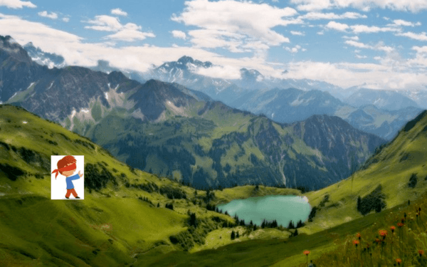
The rough terrain is analogous to the cost function. Minimizing the cost function is analogous to trying to reach lower altitudes. You are blind folded, since we don’t have the luxury of evaluating (seeing) the value of the function for every possible set of parameters. Feeling the slope of the terrain around you is analogous to calculating the gradient, and taking a step is analogous to one iteration of update to the parameters.
By the way — as a small aside — this tutorial is part of the free Data Science Course and free Machine Learning Course on Commonlounge. The courses include many hands-on assignments and projects. If you’re interested in learning Data Science / ML, definitely recommend checking it out.
Variants of Gradient Descent
There are multiple variants of gradient descent depending on how much of the data is being used to calculate the gradient. The main reason behind these variations is computational efficiency. A dataset may have millions of data points, and calculating the gradient over the entire dataset can be computationally expensive.
- Batch gradient descent computes the gradient of the cost function w.r.t to parameter w for entire training data. Since we need to calculate the gradients for the whole dataset to perform one parameter update, batch gradient descent can be very slow.
- Stochastic gradient descent (SGD) computes the gradient for each update using a single training data point x_i (chosen at random). The idea is that the gradient calculated this way is a stochastic approximation to the gradient calculated using the entire training data. Each update is now much faster to calculate than in batch gradient descent, and over many updates, we will head in the same general direction.
- In mini-batch gradient descent, we calculate the gradient for each small mini-batch of training data. That is, we first divide the training data into small batches (say M samples / batch). We perform one update per mini-batch. M is usually in the range 30–500, depending on the problem. Usually mini-batch GD is used because computing infrastructure - compilers, CPUs, GPUs - are often optimized for performing vector additions and vector multiplications.
Of these, SGD and mini-batch GD are most popular. In a typical scenario, we do several passes over the training data before the termination criteria is met. Each pass is called an epoch. Also note that since the update step is much more computationally efficient in SGD and mini-batch GD, we typically perform 100s-1000s of updates in between checks for termination criteria being met.
Choosing the learning rate
Typically, the value of the learning rate is chosen manually. We usually start with a small value such as 0.1, 0.01 or 0.001 and adapt it based on whether the cost function is reducing very slowly (increase learning rate) or is exploding / being erratic (decrease learning rate).
Although manually choosing a learning rate is still the most common practice, several methods such as Adam optimizer, AdaGrad and RMSProp have been proposed to automatically choose a suitable learning rate.
Footnote
- The value of the gradient G depends on the inputs, the current values of the model parameters, and the cost function. You might need to revisit the topic of differentiation if you are calculating the gradient by hand.
Originally published as part of the free Machine Learning Course and free Data Science Course on www.commonlounge.com. Reposted with permission.
Related: