Building NLP Classifiers Cheaply With Transfer Learning and Weak Supervision

comments

Second Step: Building a Training Set With Snorkel

 
Building our Labeling Functions is a pretty hands-on stage, but it will pay off! I expect that if you already have domain knowledge, this should take about a day (and if you don’t then it might take a couple days.) Also, this section is a mix of what I did for my project specifically and some general advice of how to use Snorkel that you can apply to your own projects.

Since most people haven’t used Weak Supervision with Snorkel before, I’ll try to explain the approach I took in as much detail as possible. This tutorial is a good way to understand the main ideas, but reading through my workflow will hopefully save you a lot of time of trial and error.
Below is an example of a LF that returns Positive if the tweet has one of the common insults against jew. Otherwise, it abstains.

# Common insults against jews.
INSULTS = r"\bjew (bitch|shit|crow|fuck|rat|cockroach|ass|bast(a|e)rd)"

def insults(tweet_text):
    return POSITIVE if re.search(INSULTS, tweet_text) else ABSTAIN

Here’s an example of a LF that returns Negative if the tweet’s author mentions he or she is Jewish, which commonly means the tweet is not anti-semitic.

# If tweet author is Jewish then it's likely not anti-semitic.
JEWISH_AUTHOR = r"((\bI am jew)|(\bas a jew)|(\bborn a jew)"

def jewish_author(tweet_tweet):
    return NEGATIVE if re.search(JEWISH_AUTHOR, tweet_tweet) else ABSTAIN

When designing LFs it’s important to keep in mind that we are prioritizing high precision over recall. Our hope is that the classifier will pick up more patterns, increasing recall. But, don’t worry if LFs don’t have super high precision or high recall, Snorkel will take care of it.
Once you have some LFs, you just need to build a matrix with a tweet in each row and the LF values in the columns. Snorkel Metal has a very handy util function to display a summary of your LFs.

# We build a matrix of LF votes for each tweet
LF_matrix = make_Ls_matrix(LF_set, LFs)

# Get true labels for LF set
Y_LF_set = np.array(LF_set['label'])

display(lf_summary(sparse.csr_matrix(LF_matrix), 
                   Y=Y_LF_set, 
                   lf_names=LF_names.values()))

I have a total of 24 LFs, but here’s how the LF summary looks like for a sample of my LFs. Below the table you can find what each column means.

LF Summary

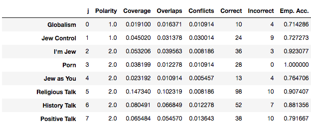
Column meanings:

• Emp. Accuracy: fraction of correct LF predictions. You should make sure this is at least 0.5 for all LFs.
• Coverage: % of samples for which at least one LF votes positive or negative. You want to maximize this, while keeping a good accuracy.
• Polarity: tells you what values the LF returns.
• Overlaps & Conflicts: this tells you how an LF overlaps and conflicts with other LFs. Don’t worry about it too much, the Label Model will actually use this to estimate the accuracy for each LF.

Let’s check out our coverage:

label_coverage(LF_matrix)
>> 0.8062755798090041

That’s pretty good!

Now, as a baseline for our weak supervision, we’ll evaluate our LFs by using a Majority Label Voter model to predict the classes in our LF set. This just assigns a positive label if most of the LFs are positive, so it’s basically assuming that all LFs have the same accuracy.

from metal.label_model.baselines import MajorityLabelVoter

mv = MajorityLabelVoter()
Y_train_majority_votes = mv.predict(LF_matrix)
print(classification_report(Y_LFs, Y_train_majority_votes))

Classification Report for Majority Voter Baseline

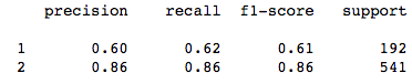
We can see that we get an F1-score of 0.61 for the positive class (“1”). To improve this, I made a spreadsheet where each row has a tweet, its true label, its assigned label based on each LF. The goal is to find where an LF disagrees with the true label, and fix the LF accordingly.

Google Sheet I used for tuning my LFs

After my LFs had about 60% precision and 60% recall, I went ahead and trained the Label Model.

Ls_train = make_Ls_matrix(train, LFs)

# You can tune the learning rate and class balance.
label_model = LabelModel(k=2, seed=123)
label_model.train_model(Ls_train, n_epochs=2000, print_every=1000, 
                        lr=0.0001, 
                        class_balance=np.array([0.2, 0.8]))

Now to test the Label Model, I validated it against my test set and plotted a Precision-Recall curve. We can see that we are able to get about 80% precision and 20% recall, which is pretty good. A big advantage of using the Label Model is that we can now tune the prediction probability threshold to get better precision.

Precision-Recall Curve for Label Model

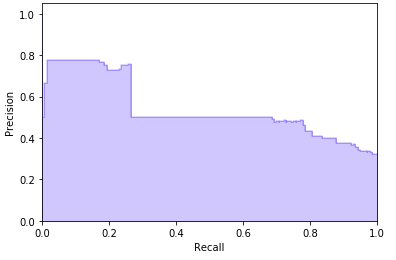
I also validated my Label Model was working by checking the top 100 most anti-semitic tweets in my train set according to the Label Model and making sure it made sense. Now that we are happy with our Label Model, we produce our training labels:

# To use all information possible when we fit our classifier, we can # actually combine our hand-labeled LF set with our training set.

Y_train = label_model.predict(Ls_train) + Y_LF_set

So, here’s a summary of my WS workflow:

1. Go through the examples in the LF set and identify a new potential LF.
2. Add it to the Label Matrix and check that its accuracy is at least 50%. Try to get the highest accuracy possible, while keeping a good coverage. I grouped different LFs together if they relate to the same topic.
3. Every once in a while you’ll want to use the baseline Majority Vote model (provided in Snorkel Metal) to label your LF set. Update your LFs accordingly to get a pretty good score just with the Majority Vote model.
4. If your Majority Vote model isn’t good enough, then you can fix your LFs or go back to step 1 and repeat.
5. Once your Majority Vote model works, then run your LFs over your Train set. You should have at least 60% coverage.
6. Once this is done, train your Label Model!
7. To validate the Label Model, I ran the Label Model over my Training set and printed the top 100 most anti-semitic tweets and 100 least anti-semitic tweets to make sure it was working correctly.

Now that we have our Label Model, we can compute probabilistic labels for 25 thousand of tweets and use them as a training set. Now, let’s go ahead and train our classification model!

General Tips for Snorkel:

• On LF accuracy: In the WS step, we’re going for high precision. All of your LFs should have at least 50% accuracy on the LF set. If you can get 75% or more that’s even better.
• On LF coverage: You want to have at least one LF voting positive/negative for at least 65% of our training set. This is called LF Coverage by Snorkel.
• If you’re not a domain expert to start, you’ll get ideas for new LFs as you label your 600 initial data points.

Third Step: Build Classification Model

 
The last step is to train our classifier to generalize beyond our noisy hand-made rules.

Baselines

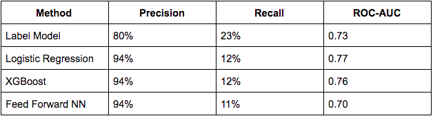
We’ll start by setting some baselines. I tried to build the best model possible without deep learning. I tried Tf-idf featurization coupled with logistic regression from sklearn, XGBoost, and Feed Forward Neural Networks.

Below are the results. To get these numbers I plotted a Precision-Recall curve against the Development set, and then picked my preferable classification threshold (trying to get a minimum of 90% precision if possible with recall as high as possible).

Baselines

Trying ULMFiT

Once we download the ULM trained on Wikipedia, we need to tune it to tweets since they have a pretty different language. I followed all the steps and code in this awesome blog, and I also used the Twitter Sentiment140 datasetfrom Kaggle to fine-tune the LM.

We sample 1 million tweets from that dataset randomly, and fine-tune the LM on those tweets. This way, the LM will learn be able to generalize in the twitter domain.
The code below loads the tweets and trains the LM. I used a GPU from Paperspace using the fastai public image, this worked wonders. You can follow these steps to set it up.

data_lm = TextLMDataBunch.from_df(train_df=LM_TWEETS,         valid_df=df_test, path="")

learn_lm = language_model_learner(data_lm, pretrained_model=URLs.WT103_1, drop_mult=0.5)

We unfreeze all the layers in the LM:

learn_lm.unfreeze()

We let it run for 20 cycles. I put the cycles in a for loop so that I could save the model after every iteration. I didn’t find a way to do this easily with fastai.

for i in range(20):
    learn_lm.fit_one_cycle(cyc_len=1, max_lr=1e-3, moms=(0.8, 0.7))
    learn_lm.save('twitter_lm')

Then we should test the LM to make sure it’s making at least a little bit of sense:

learn_lm.predict("i hate jews", n_words=10)
>> 'i hate jews are additional for what hello you brother . xxmaj the'
learn_lm.predict("jews", n_words=10)
>> 'jews out there though probably okay jew back xxbos xxmaj my'

The weird tokens like “xxmaj” are some special tokens that fastai adds that help with text understanding. For example, they add special tokens for capital letters, beginning of a sentence, repeated words, etc. The LM is not really making that much sense, but that’s fine.
Now we’ll train our classifier:

# Classifier model data
data_clas = TextClasDataBunch.from_df(path = "", 
                                      train_df = df_trn,
                                      valid_df = df_val,                                         
                                      vocab=data_lm.train_ds.vocab, 
                                      bs=32, 
                                      label_cols=0)

learn = text_classifier_learner(data_clas, drop_mult=0.5)
learn.freeze()

Using fastai’s method for finding a good learning rate:

learn.lr_find(start_lr=1e-8, end_lr=1e2)
learn.recorder.plot()

We’ll fine-tune the classifier with gradual unfreezing:

learn.fit_one_cycle(cyc_len=1, max_lr=1e-3, moms=(0.8, 0.7))
learn.freeze_to(-2)
learn.fit_one_cycle(1, slice(1e-4,1e-2), moms=(0.8,0.7))
learn.freeze_to(-3)
learn.fit_one_cycle(1, slice(1e-5,5e-3), moms=(0.8,0.7))
learn.unfreeze()
learn.fit_one_cycle(4, slice(1e-5,1e-3), moms=(0.8,0.7))

A few training epochs

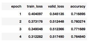
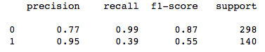
After fine-tuning, let’s plot our Precision-Recall curve! It was very nice to see this after the first try.

Precision-Recall curve of ULMFiT with Weak Supervision

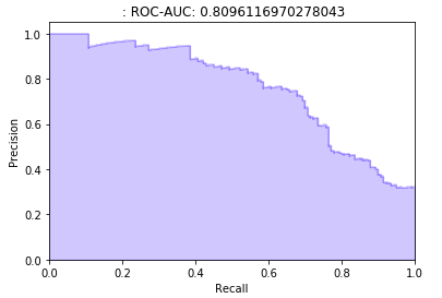
I picked probability threshold of 0.63, which gives us 95% precision and 39% recall. This is a very large boost mainly in recall but also in precision.

Classification Report for ULMFiT Model

Having Fun With Our Model

Below is a pretty cool example of how the model catches that “doesn’t” changes the tweet’s meaning!

learn.predict("george soros controls the government")
>> (Category 1, tensor(1), tensor([0.4436, 0.5564]))

learn.predict("george soros doesn't control the government")
>> (Category 0, tensor(0), tensor([0.7151, 0.2849]))

Here are some insults against jews:

learn.predict("fuck jews")
>> (Category 1, tensor(1), tensor([0.1996, 0.8004]))

learn.predict("dirty jews")
>> (Category 1, tensor(1), tensor([0.4686, 0.5314]))

Here is a person calling out anti-semitic tweets:

learn.predict("Wow. The shocking part is you're proud of offending every serious jew, mocking a religion and openly being an anti-semite.")
>> (Category 0, tensor(0), tensor([0.9908, 0.0092]))

And here are other non anti-semitic tweets:

learn.predict("my cousin is a russian jew from ukraine- ???????????? i'm so glad they here")
>> (Category 0, tensor(0), tensor([0.8076, 0.1924]))

learn.predict("at least the stolen election got the temple jew shooter off the drudgereport. I ran out of tears.")
>> (Category 0, tensor(0), tensor([0.9022, 0.0978]))

Does Weak Supervision Actually Help?

I was curious if WS was necessary to obtain this performance, so I ran a little experiment. I ran the same process as before, but without the WS labels, and got this Precision-Recall curve:

Precision-Recall curve of ULMFiT without Weak Supervision

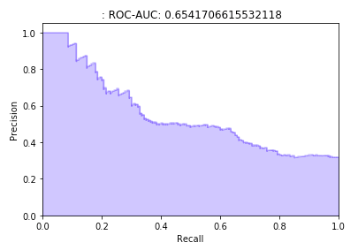
We can see a big drop in recall (we only get about 10% recall for a 90% precision) and ROC-AUC (-0.15), compared to the previous Precision-Recall curve in which we used our WS labels.

Conclusions

• Weak supervision + ULMFiT helped us hit 95% precision and 39% recall. That was much better than all the baselines, so that was very exciting. I was not expecting that at all.
• This model is very easy to keep up-to-date. There’s no need for relabeling, we just update the LFs and rerun the WS + ULMFiT pipeline.
• Weak supervision makes a big difference by allowing ULMFiT to generalize better.

Next Steps

• I believe we can get the most gains by putting some more effort into my LFs to improve the Weak Supervision model. I would first include LFs based on external knowledge bases like Hatebase’s repository of hate speech patterns. Then, I would write new LFs based on Spacy’s dependency tree parsing.
• We didn’t do any hyperparameter tuning but that could likely help improve both the Label Model and ULMFiT performance.
• We can try different classification models such as fine-tuning BERT or OpenAI’s Transformer.

 
Bio: Abraham Starosta (starosta@stanford.edu) is originally from Venezuela and is now finishing his Master's in Computer Science at Stanford University, focusing in AI and NLP. Prior to starting his Master's at Stanford, he was a Data Scientist at Primer AI, a startup building text understanding and summarization technologies. He was a co-founder of Nav Talent, a technical recruiting agency for top startups that started at Stanford. Over the years, he also had the opportunity to be a software engineer at other top startups like Livongo, Zugata and Splunk. In his spare time he enjoys playing soccer and ping pong.

Original. Reposted with permission.

Related:

• How to solve 90% of NLP problems: a step-by-step guide
• OpenAI’s GPT-2: the model, the hype, and the controversy
• More Effective Transfer Learning for NLP