 The Most Important Fundamentals of PyTorch you Should Know
 The Most Important Fundamentals of PyTorch you Should Know
PyTorch is a constantly developing deep learning framework with many exciting additions and features. We review its basic elements and show an example of building a simple Deep Neural Network (DNN) step-by-step.

Fundamentals of PyTorch – Introduction
Since it was introduced by the Facebook AI Research (FAIR) team, back in early 2017, PyTorch has become a highly popular and widely used Deep Learning (DL) framework. Since the humble beginning, it has caught the attention of serious AI researchers and practitioners around the world, both in industry and academia, and has matured significantly over the years.
Scores of DL enthusiasts and professionals started their journey with the Google TensorFlow (TF), but the learning curve with base TensorFlow has always been steep. On the other hand, PyTorch has approached DL programming in an intuitive fashion since the beginning, focusing on fundamental linear algebra and data flow operations in a manner that is easily understood and amenable to step-by-step learning.
Due to this modular approach, building and experimenting with complex DL architectures has been much easier with PyTorch than following the somewhat rigid framework of TF and TF-based tools. Moreover, PyTorch was built to integrate seamlessly with the numerical computing infrastructure of the Python ecosystem and Python being the lingua franca of data science and machine learning, it has ridden over that wave of increasing popularity.
Tensor Operations with PyTorch
Tensors are at the heart of any DL framework. PyTorch provides tremendous flexibility to a programmer about how to create, combine, and process tensors as they flow through a network (called computational graph) paired with a relatively high-level, object-oriented API.
What are Tensors?
Representing data (e.g., about the physical world or some business process) for Machine Learning (ML), in particular for DNN, is accomplished via a data/mathematical structure known as the tensor. A tensor is a container that can house data in N dimensions. A tensor is often used interchangeably with another more familiar mathematical object matrix (which is specifically a 2-dimensional tensor). In fact, tensors are generalizations of 2-dimensional matrices to N-dimensional space.
In simplistic terms, one can think of scalar-vectors-matrices- tensors as a flow.
- Scalar are 0-dimensional tensors.
- Vectors are 1-dimensional tensors.
- Matrices are 2-dimensional tensors
- Tensors are generalized N-dimensional tensors. N can be anything from 3 to infinity…
Often, these dimensions are also called ranks.
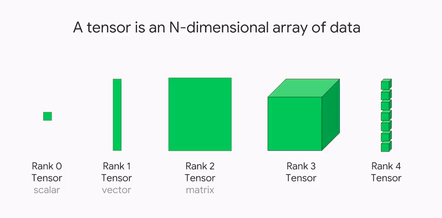
Fig 1: Tensors of various dimensions (ranks) (Image source).
Why Are Tensors Important for ML and DL?
Think of a supervised ML problem. You are given a table of data with some labels (could be numerical entities or binary classification such as Yes/No answers). For ML algorithms to process it, the data must be fed as a mathematical object. A table is naturally equivalent to a 2-D matrix where an individual row (or instance) or individual column (or feature) can be treated as a 1-D vector.
Similarly, a black-and-white image can be treated as a 2-D matrix containing numbers 0 or 1. This can be fed into a neural network for image classification or segmentation tasks.
A time-series or sequence data (e.g., ECG data from a monitoring machine or a stock market price tracking data stream) is another example of 2-D data where one dimension (time) is fixed.
These are examples of using 2-D tensors in classical ML (e.g., linear regression, support vector machines, decision trees, etc.) and DL algorithms.
Going beyond 2-D, a color or grayscale image can be treated as a 3-D tensor where each pixel is associated with a so-called ‘color-channel’ – a vector of 3 numbers representing intensities in the Red-Green-Blue (RGB) spectrum. This is an example of a 3-D tensor.
Similarly, videos can be thought of as sequences of color images (or frames) in time and can be thought of as 4-D tensors.
In short, all kinds of data from the physical world, sensors and instruments, business and finance, scientific or social experiments, can be easily represented by multi-dimensional tensors to make them amenable for processing by ML/DL algorithms inside a computing machine.
Let’s see how PyTorch defines and handles tensors.
Creating and Converting Tensors in PyTorch
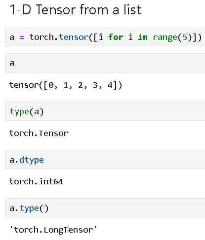
Tensors can be defined from a Python list as follows,
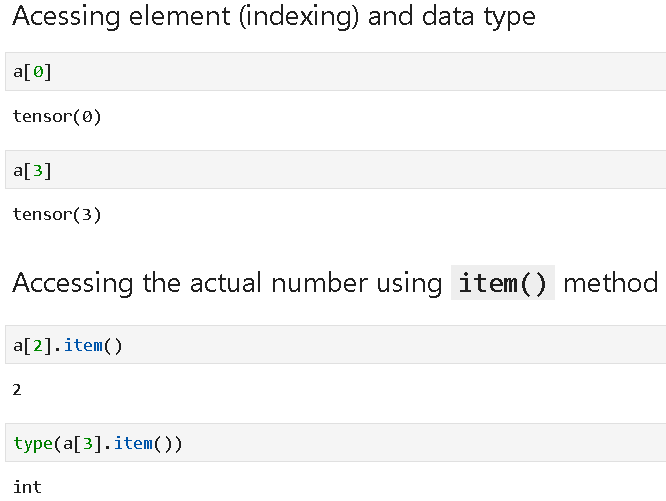
Actual elements can be accessed and indexed as follows,
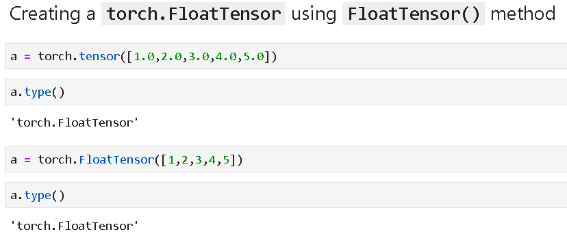
Tensors with specific data types can be created easily (e.g., floating points),
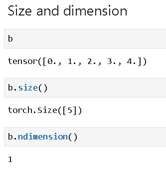
Size and dimensions can be read easily,
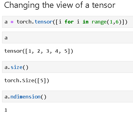
We can change the view of a tensor. Let us start with a 1-dimensional tensor as follows,
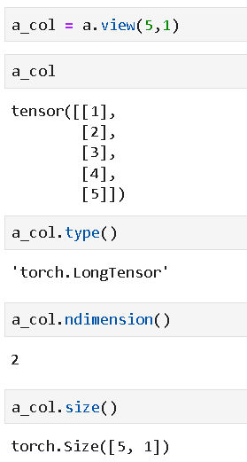
Then change the view to a 2-D tensor,
Changing back and forth between a PyTorch tensor and a NumPy array is easy and efficient.

Converting from a Pandas series object is also easy,

Finally, converting back to a Python list can be accomplished,

Vector and matrix mathematics with PyTorch tensors
PyTorch provides an easy-to-understand API and programmatic toolbox to manipulate tensors mathematically. We show basic operations with 1-D and 2-D tensors here.
Simple vector addition,

Vector multiplication with a scalar,

Linear combination,

Element-wise product,

Dot product,

Adding a scalar to every element of a tensor, i.e., broadcasting,

Creating 2-D tensor from list of lists,

Slicing and indexing of matrix elements,

Matrix multiplication,

Matrix transpose,

Matrix inverse and determinant,

Autograd: Automatic differentiation
Neural network training and prediction involves taking derivatives of various functions (tensor-valued) over and over. The Tensor object supports the magical Autograd feature, i.e., automatic differentiation, which is achieved by tracking and storing all the operations performed on the tensor while it flows through a network. You can watch this wonderful tutorial video for a visual explanation:
The Pytorch autograd official documentation is here.
We show simple examples to illustrate the autograd feature of PyTorch.

We define a generic function and a tensor variable x, then define another variable y assigning it to the function of x.

Then, we use a special backward() method on y to take the derivative and calculate the derivative value at the given value of x.

We can also deal with partial derivatives!

We can define u and v as tensor variables, define a function combining them, apply the backward() method, and calculate the partial derivatives. See below,

PyTorch computes derivatives of scalar functions only, but if we pass a vector, then essentially it computes derivatives element-wise and stores them in an array of the same dimension.

The following code will calculate the derivative with respect to the three constituent vectors.

We can show the plot of the derivative. Note, a derivative of a quadratic function is a straight line, tangent to the parabolic curve.

Building a Full-Fledged Neural Network
Apart from the tensors and automatic differentiation ability, there are few more core components/features of PyTorch that come together for a deep neural network definition.
The core components of PyTorch that will be used for building the neural classifier are,
- The Tensor (the central data structure in PyTorch)
- The Autograd feature of the Tensor (automatic differentiation formula baked into the
- The nn.Module class that is used to build any other neural classifier class
- The Optimizer (of course, there are many of them to choose from)
- The Loss function (a big selection is available for your choice)
We have already described in detail the Tensor and the Autograd. Let us quickly discuss the other components,
The nn.Module Class
In PyTorch, we construct a neural network by defining it as a custom class. However, instead of deriving from the native Python object, this class inherits from the nn.Module class. This imbues the neural net class with useful properties and powerful methods. This way, the full power of Object-Oriented-Programming (OOP) can be maintained while working with neural net models. We will see a full example of such a class definition in our article.
The Loss Function
In a neural network architecture and operation, the loss functions define how far the final prediction of the neural net is from the ground truth (given labels/classes or data for supervised training). The quantitative measure of loss helps drive the network to move closer to the configuration (the optimal settings of the weights of the neurons), which classifies the given dataset best or predicts the numerical output with the least total error.
PyTorch offers all the usual loss functions for classification and regression tasks —
- binary and multi-class cross-entropy,
- mean squared and mean absolute errors,
- smooth L1 loss,
- neg log-likelihood loss, and even
- Kullback-Leibler divergence.
A detailed discussion of these can be found in this article.
The Optimizer
Optimization of the weights to achieve the lowest loss is at the heart of the backpropagation algorithm for training a neural network. PyTorch offers a plethora of optimizers to do the job, exposed through the torch.optim module —
- Stochastic gradient descent (SGD),
- Adam, Adadelta, Adagrad, SpareAdam,
- L-BFGS,
- RMSprop, etc.
Look at this article to know more about activation functions and optimizers, used in modern deep neural networks.
The Five-Step-Process
Using these components, we will build the classifier in five simple steps,
- Construct our neural network as our custom class (inherited from the nn.Module class), complete with hidden layer tensors and forward method for propagating the input tensor through various layers and activation function
- Propagate the feature (from a dataset) tensor through the network using this forward() method — say we get an output tensor as a result
- Calculate the loss by comparing the output to the ground truth and using built-in loss functions
- Propagate the gradient of the loss using the automatic differentiation ability (Autograd) with the backward method
- Update the weights of the network using the gradient of the loss — this is accomplished by executing one step of the so-called optimizer — optimizer.step().
And that’s it. This five-step process constitutes one complete epoch of training. We just repeat it a bunch of times to drive down the loss and obtain high classification accuracy.
The idea looks like following,

Hands-on example
Let’s suppose we want to build and train the following 2-layer neural network.

We start with the class definition,

We can define a variable as an object belonging to this class and print the summary.

We choose the Binary cross-entropy loss,

Let us run the input dataset through the neural net model we have defined, i.e., forward pass once and compute the output probabilities. As the weights have been initialized as random, we will see random output probabilities (mostly close to 0.5). This network has not been trained yet.


We define the optimizer,

Next, we show how to do forward and backward passes with one step of optimizer. This set of code can be found at the heart of any PyTorch neural net model. We follow another five-step process,
- reset the gradients to zero (to prevent the accumulation of grads)
- forward pass the tensors through the layers
- calculate the loss tensor
- calculate the gradients of the loss
- update the weights by incrementing the optimizer by one step (in the direction of the negative gradient)
The five steps above are exactly what you can observe and read about in all the theoretical discussion (and in the textbooks) on neural nets and deep learning. And, with PyTorch, you are able to implement this process with deceptively simple code, step-by-step.
The code is shown below,

When we run the same type of code over a loop (for multiple epochs), we can observe the familiar loss-curve going down, i.e., the neural network getting trained gradually.

After training for 200 epochs, we can look at the probability distributions again directly to see how the neural network output probabilities are now different (trying to match with the true data distributions).

Summary of PyTorch Fundamentals
PyTorch is a great package for reaching out to the heart of a neural net and customizing it for your application or trying out bold new ideas with the architecture, optimization, and mechanics of the network.
You can easily build complex interconnected networks, try out novel activation functions, mix and match custom loss functions, etc. The core ideas of computation graphs, easy auto-differentiation, and forward and backward flow of tensors will come in handy for any of your neural network definitions and optimization.
In this article, we summarized a few key steps which can be followed to quickly build a neural network for classification or regression tasks. We also showed how neat ideas could be easily tried out with this framework.
All the code for this article can be found here in this Github repo.
Original. Reposted with permission.
Related: