Preprocessing for Deep Learning: From covariance matrix to image whitening

comments

3. Image whitening

 
We will see how whitening can be applied to preprocess an image dataset. To do so we will use the paper of Pal & Sudeep (2016) where they give some details about the process. This preprocessing technique is called Zero component analysis (ZCA).

Check out the paper, but here is the kind of result they got. The original images (left) and the images after the ZCA (right) are shown.

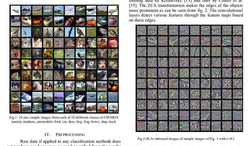
Whitening images from the CIFAR10 dataset. Results from the paper of Pal & Sudeep (2016).

First things first. We will load images from the CIFAR dataset. This dataset is available from Keras and you can also download it here.

(50000, 32, 32, 3)

The training set of the CIFAR10 dataset contains 50000 images. The shape of X_train is (50000, 32, 32, 3). Each image is 32px by 32px and each pixel contains 3 dimensions (R, G, B). Each value is the brightness of the corresponding color between 0 and 255.

We will start by selecting only a subset of the images, let’s say 1000:

(1000, 32, 32, 3)

That’s better. Now we will reshape the array to have flat image data with one image per row. Each image will be (1, 3072) because 32 x 32 x 3 = 3072. Thus, the array containing all images will be (1000, 3072):

(1000, 3072)

The next step is to be able to see the images. The function imshow() from Matplotlib (doc) can be used to show images. It needs images with the shape (M x N x 3) so let’s create a function to reshape the images and be able to visualize them from the shape (1, 3072).

For instance, let’s plot one of the images we have loaded:

Cute!
We can now implement the whitening of the images. Pal & Sudeep (2016)describe the process:

1. The first step is to rescale the images to obtain the range [0, 1] by dividing by 255 (the maximum value of the pixels).

Recall that the formula to obtain the range [0, 1] is:

but, here, the minimum value is 0, so this leads to:

X.min() 0.0
X.max() 1.0

Mean subtraction: per-pixel or per-image?

Ok cool, the range of our pixel values is between 0 and 1 now. The next step is:

2. Subtract the mean from all images.

Be careful here.

One way to do it is to take each image and remove the mean of this image from every pixel (Jarrett et al., 2009). The intuition behind this process is that it centers the pixels of each image around 0.

Another way to do it is to take each of the 3072 pixels that we have (32 by 32 pixels for R, G and B) for every image and subtract the mean of that pixel across all images. This is called per-pixel mean subtraction. This time, each pixel will be centered around 0 according to all images. When you will feed your network with the images, each pixel is considered as a different feature. With the per-pixel mean subtraction, we have centered each feature (pixel) around 0. This technique is commonly used (e.g Wan et al., 2013).

We will now do the per-pixel mean subtraction from our 1000 images. Our data are organized with these dimensions (images, pixels). It was (1000, 3072) because there are 1000 images with 32 x 32 x 3 = 3072 pixels. The mean per-pixel can thus be obtained from the first axis:

(3072,)

This gives us 3072 values which is the number of means — one per pixel. Let’s see the kind of values we have:

array([ 0.5234 , 0.54323137, 0.5274 , …, 0.50369804,
 0.50011765, 0.45227451])

This is near 0.5 because we already have normalized to the range [0, 1]. However, we still need to remove the mean from each pixel:

Just to convince ourselves that it worked, we will compute the mean of the first pixel. Let’s hope that it is 0.

array([ -5.30575583e-16, -5.98021632e-16, -4.23439062e-16, …,
 -1.81965554e-16, -2.49800181e-16, 3.98570066e-17])

This is not exactly 0 but it is small enough that we can consider that it worked!

Now we want to calculate the covariance matrix of the zero-centered data. Like we have seen above, we can calculate it with the np.cov() function from NumPy.

There are two possible correlation matrices that we can calculate from the matrix X: either the correlation between rows or between columns. In our case, each row of the matrix X is an image, so the rows of the matrix correspond to the observations and the columns of the matrix corresponds to the features (the images pixels). We want to calculate the correlation between the pixels because the goal of the whitening is to remove these correlations to force the algorithm to focus on higher-order relations.

To do so, we will tell this to Numpy with the parameter rowvar=False (see the doc): it will use the columns as variables (or features) and the rows as observations.

cov = np.cov(X_norm, rowvar=False)

The covariance matrix should have a shape of 3072 by 3072 to represent the correlation between each pair of pixels (and there are 3072 pixels):

cov.shape

(3072, 3072)

Now the magic part — we will calculate the singular values and vectors of the covariance matrix and use them to rotate our dataset. Have a look at my poston the singular value decomposition (SVD)if you need more details.

Note: It can take a bit of time with a lot of images and that's why we are using only 1000. In the paper, they used 10000 images. Feel free to compare the results according to how many images you are using:

In the paper, they used the following equation:

with U the left singular vectors and S the singular values of the covariance of the initial normalized dataset of images, and X the normalized dataset. ϵ is an hyper-parameter called the whitening coefficient. diag(a) corresponds to a matrix with the vector a as a diagonal and 0 in all other cells.

We will try to implement this equation. Let’s start by checking the dimensions of the SVD:

(3072, 3072) (3072,)

S is a vector containing 3072 elements (the singular values). diag(S) will thus be of shape (3072, 3072) with S as the diagonal:

[[ 8.15846654e+00 0.00000000e+00 0.00000000e+00 …, 0.00000000e+00
 0.00000000e+00 0.00000000e+00]
 [ 0.00000000e+00 4.68234845e+00 0.00000000e+00 …, 0.00000000e+00
 0.00000000e+00 0.00000000e+00]
 [ 0.00000000e+00 0.00000000e+00 2.41075267e+00 …, 0.00000000e+00
 0.00000000e+00 0.00000000e+00]
 …, 
 [ 0.00000000e+00 0.00000000e+00 0.00000000e+00 …, 3.92727365e-05
 0.00000000e+00 0.00000000e+00]
 [ 0.00000000e+00 0.00000000e+00 0.00000000e+00 …, 0.00000000e+00
 3.52614473e-05 0.00000000e+00]
 [ 0.00000000e+00 0.00000000e+00 0.00000000e+00 …, 0.00000000e+00
 0.00000000e+00 1.35907202e-15]]

shape: (3072, 3072)

Check this part:

is also of shape (3072, 3072) as well as U and U^T. We have seen also that X has the shape (1000, 3072) and we need to transpose it to have (3072, 1000). The shape of X_ZCA is thus:

which corresponds to the shape of the initial dataset. Nice.

We have:

epsilon = 0.1
X_ZCA = U.dot(np.diag(1.0/np.sqrt(S + epsilon))).dot(U.T).dot(X_norm.T).T

Let's rescale the images:

X_ZCA_rescaled = (X_ZCA - X_ZCA.min()) / (X_ZCA.max() - X_ZCA.min())
print 'min:', X_ZCA_rescaled.min()
print 'max:', X_ZCA_rescaled.max()

min: 0.0
max: 1.0

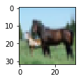
Finally, we can look at the effect of whitening by comparing an image before and after whitening:

plotImage(X[12, :])
plotImage(X_ZCA_rescaled[12, :])

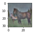
Hooray! That's great! looks like the images from the paper Pal & Sudeep (2016). They used epsilon = 0.1. You can try other values to see the effect on the image.

That's all!

I hope that you found something interesting in this article You can read it on my blog, with LaTeX for the math, along with other articles.

You can also fork the Jupyter notebook on Github here.

References

K. Jarrett, K. Kavukcuoglu, M. Ranzato, and Y. LeCun, “What is the best multi-stage architecture for object recognition?,” in 2009 IEEE 12th International Conference on Computer Vision, 2009, pp. 2146–2153.

A. Krizhevsky, “Learning Multiple Layers of Features from Tiny Images,” Master’s thesis, University of Tront, 2009.

Y. A. LeCun, L. Bottou, G. B. Orr, and K.-R. Müller, “Efficient BackProp,” in Neural Networks: Tricks of the Trade, Springer, Berlin, Heidelberg, 2012, pp. 9–48.

K. K. Pal and K. S. Sudeep, “Preprocessing for image classification by convolutional neural networks,” in 2016 IEEE International Conference on Recent Trends in Electronics, Information Communication Technology (RTEICT), 2016, pp. 1778–1781.

L. Wan, M. Zeiler, S. Zhang, Y. L. Cun, and R. Fergus, “Regularization of Neural Networks using DropConnect,” in International Conference on Machine Learning, 2013, pp. 1058–1066.

Great resources and QA

Wikipedia — Whitening transformation

CS231 — Convolutional Neural Networks for Visual Recognition

Dustin Stansbury — The Clever Machine

Some details about the covariance matrix

SO — Image whitening in Python

Mean normalization per image or from the entire dataset

Mean subtraction — all images or per image?

Why centering is important — See section 4.3

Kaggle kernel on ZCA

How ZCA is implemented in Keras

 
Bio: Hadrien Jean is a machine learning scientist. He owns a Ph.D in cognitive science from the Ecole Normale Superieure, Paris, where he did research on auditory perception using behavioral and electrophysiological data. He previously worked in industry where he built deep learning pipelines for speech processing. At the corner of data science and environment, he works on projects about biodiversity assessement using deep learning applied to audio recordings. He also periodically creates content and teaches at Le Wagon (data science Bootcamp), and writes articles in his blog (hadrienj.github.io).

Original. Reposted with permission.

Related:

• Basic Image Data Analysis Using Numpy and OpenCV – Part 1
• Basic Image Processing in Python, Part 2
• 7 Steps to Mastering Data Preparation with Python