Classifying Heart Disease Using K-Nearest Neighbors

comments

Building Heart disease classifier using K-NN algorithm

source

The most crucial task in the healthcare field is disease diagnosis. If a disease is diagnosed early, many lives can be saved. Machine learning classification techniques can significantly benefit the medical field by providing an accurate and quick diagnosis of diseases. Hence, save time for both doctors and patients. As heart disease is the number one killer in the world today, it becomes one of the most difficult diseases to diagnose.

In this section, we are going to build a K-NN classifier which will predict the presence of heart disease in a patient or not.

You can download the dataset from the UCI Machine Learning repository.

This database contains 76 attributes, but all published experiments refer to using a subset of 14 of them. In particular, the Cleveland database is the only one that has been used by ML researchers to this date. The “goal” field refers to the presence of heart disease in the patient. It is integer valued from 0 (no presence) to 4.

Dataset contains following features:

age — age in years
sex — (1 = male; 0 = female)
cp — chest pain type
trestbps — resting blood pressure (in mm Hg on admission to the hospital)
chol — serum cholestoral in mg/dl
fbs — (fasting blood sugar > 120 mg/dl) (1 = true; 0 = false)
restecg — resting electrocardiographic results
thalach — maximum heart rate achieved
exang — exercise induced angina (1 = yes; 0 = no)
oldpeak — ST depression induced by exercise relative to rest
slope — the slope of the peak exercise ST segment
ca — number of major vessels (0–3) colored by flourosopy
thal — 3 = normal; 6 = fixed defect; 7 = reversable defect
target — have disease or not (1=yes, 0=no)

Lets load all the required libraries.

import numpy as np
import matplotlib.pyplot as plt 
import pandas as pd
import seaborn as sns
from sklearn.model_selection import train_test_split
from sklearn.preprocessing import StandardScaler
from sklearn.neighbors import KNeighborsClassifier
from sklearn.metrics import confusion_matrix
from sklearn import metrics

Let's load our dataset:

data = pd.read_csv('/Users/nageshsinghchauhan/Downloads/ML/KNN_art/heart.csv')

Our original data set looks like this

 
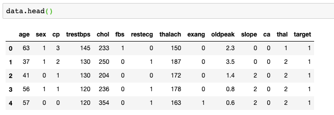
Let us explore our dataset and count the number of patients who have heart disease:

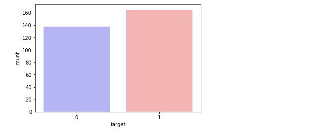
data.target.value_counts()

1    165
0    138
Name: target, dtype: int64

So out of all the patients 165 patients actually have heart disease. Now also visualize.

sns.countplot(x="target", data=data, palette="bwr")
plt.show()

count of the number of patients having heart disease(target =1)

Now let's classify target variable between male and female and visualize the result.

sns.countplot(x='sex', data=data, palette="mako_r")
plt.xlabel("Sex (0 = female, 1= male)")
plt.show()

count of the male and female having heart disease

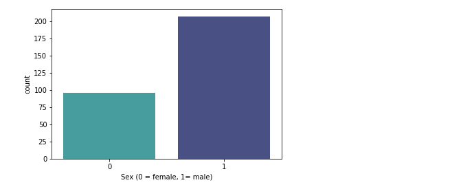
So from the above figure, it is evident that in our dataset, 207 males and 96 females are there.

Let us also see the relation between “Maximum Heart Rate” and “Age”.

plt.scatter(x=data.age[data.target==1], y=data.thalach[(data.target==1)], c="green")
plt.scatter(x=data.age[data.target==0], y=data.thalach[(data.target==0)], c = 'black')
plt.legend(["Disease", "Not Disease"])
plt.xlabel("Age")
plt.ylabel("Maximum Heart Rate")
plt.show()

Scatter plot between Age and Maximum heart rate

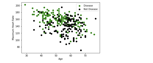
So from the above, the maximum heart rate occurs in between age 50–60 years.

Ok, now let's label our dataset with X(matrix of independent variables) and y(vector of the dependent variable).

X = data.iloc[:,:-1].values
y = data.iloc[:,13].values

Next, we split 75% of the data to the training set while 25% of the data to test set using below code.

X_train, X_test, y_train, y_test =  train_test_split(X,y,test_size = 0.25, random_state= 0)

Now, Our dataset contains features which are highly varying in magnitudes, units, and range. But since most of the machine learning algorithms use Euclidean distance between two data points in their computations, this is a problem. To suppress this effect, we need to bring all features to the same level of magnitudes. This can be achieved by a method called feature scaling.

So our next step is to normalize the data which can be done using StandardScaler() from sci-kit learn.

sc_X = StandardScaler()
X_train = sc_X.fit_transform(X_train)
X_test = sc_X.transform(X_test)

Our next step is to K-NN model and train it with the training data. Here n_neighbors is the value of factor K.

classifier = KNeighborsClassifier(n_neighbors = 5, metric = 'minkowski', p = 2)
classifier = classifier.fit(X_train,y_train)

So the most important point to note here is to choose the optimal value of K and for that, we will start with K=5.

Now, since your K-NN model is ready with K=5. Let's train our test data and check its accuracy.

y_pred = classifier.predict(X_test)
#check accuracy
accuracy = metrics.accuracy_score(y_test, y_pred)
print('Accuracy: {:.2f}'.format(accuracy))

Accuracy: 0.82

For K=6

classifier = KNeighborsClassifier(n_neighbors = 6, metric = 'minkowski', p = 2)
classifier = classifier.fit(X_train,y_train)
#prediction
y_pred = classifier.predict(X_test)
#check accuracy
accuracy = metrics.accuracy_score(y_test, y_pred)
print('Accuracy: {:.2f}'.format(accuracy))

Accuracy: 0.86

For K=7

classifier = KNeighborsClassifier(n_neighbors = 7, metric = 'minkowski', p = 2)
classifier = classifier.fit(X_train,y_train)
#prediction
y_pred = classifier.predict(X_test)
#check accuracy
accuracy = metrics.accuracy_score(y_test, y_pred)
print('Accuracy: {:.2f}'.format(accuracy))

Accuracy: 0.87

For K=8

classifier = KNeighborsClassifier(n_neighbors = 8, metric = 'minkowski', p = 2)
classifier = classifier.fit(X_train,y_train)
#prediction
y_pred = classifier.predict(X_test)
#check accuracy
accuracy = metrics.accuracy_score(y_test, y_pred)
print('Accuracy: {:.2f}'.format(accuracy))

Accuracy: 0.87

For K=9

classifier = KNeighborsClassifier(n_neighbors = 9, metric = 'minkowski', p = 2)
classifier = classifier.fit(X_train,y_train)
#prediction
y_pred = classifier.predict(X_test)
#check accuracy
accuracy = metrics.accuracy_score(y_test, y_pred)
print('Accuracy: {:.2f}'.format(accuracy))

Accuracy: 0.86

So as we can see that Accuracy is maximum that is 87% when K=7.

Let's also check the confusion matrix and see how many records were predicted correctly.

#confusion matrix
from sklearn.metrics import confusion_matrix
cm = confusion_matrix(y_test, y_pred)

array([[26, 7],
       [ 3, 40]])

In the output, 26 and 40 are correct predictions, and 7 and 3 are incorrect predictions.

How to improve the performance of your classifier?

 
Well, there are many ways in which the KNN algorithm can be improved.

• Changing the distance measure for different applications may help improve the accuracy of the algorithm. (i.e. Hamming distance for text classification).
• Dimensionality reduction techniques like PCA should be executed prior to applying K-NN
• Rescaling your data makes the distance measure more meaningful. For instance, given 2 features height and weight, an observation such as z=[220,60]z=[220,60] will clearly skew the distance metric in favor of height. One way of fixing this is by column-wise subtracting the mean and dividing by the standard deviation.
• Approximate Nearest Neighbor techniques such as using k-d trees to store the training data can be performed to decrease testing time.

Conclusion

 
Congratulations, you have successfully built a heart disease classifier using K-NN which is capable of classifying heart patient with optimal accuracy.

In this article, we have learned the K-NN, it’s working, the curse of dimensionality, model building and evaluation on heart disease dataset using Python Scikit-learn package.

Well, I hope you guys have enjoyed reading this article. Let me know your thoughts/suggestions/questions in the comment section.

You can reach me out on LinkedIn for any query.

Thanks for reading !!!

 
Bio: Nagesh Singh Chauhan is a Big data developer at CirrusLabs. He has over 4 years of working experience in various sectors like Telecom, Analytics, Sales, Data Science having specialisation in various Big data components.

Original. Reposted with permission.

Related:

• A Beginner’s Guide to Linear Regression in Python with Scikit-Learn
• Build Your First Chatbot Using Python & NLTK
• Predict Age and Gender Using Convolutional Neural Network and OpenCV